
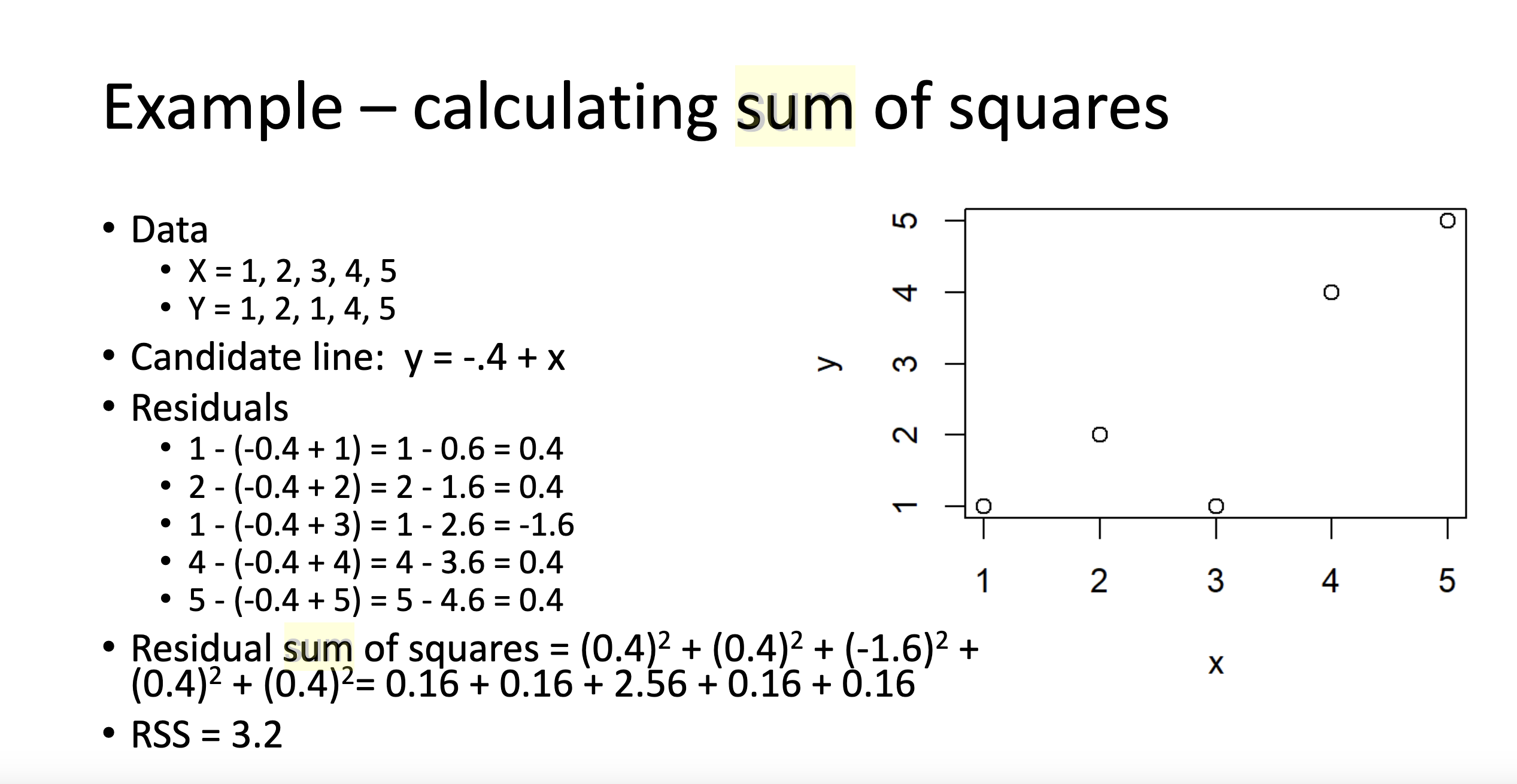
x <- "Hello World"
# anything I write after the "#" will not be executed
print(x) # this code will tell R to print the object x.
[1] "Hello World"This page is my own personal recitation website. I will post both course material and anything we go over in recitation. This is simply a central hub that you can use to help you throughout the semester.
This does not replace the lecture, canvas, or your notes.
In previous years, I have used slide shows. This website is an effort to have a more organized and central workflow that is more accessible.
I teach the 017 and 018 recitation. Make sure you are in the right section!
Section 17 meets on Th 10:10am-11:01am Bruce Curtis Bldg E158
Section 18 meets on Th 1:25pm-2:15pm Clare Small Arts and Sciences 104
Pollock, Philip H. and Barry C. Edwards. 2020. The Essentials of Political Analysis. 6th Edition. CQ Press. (EPA)
Pollock, Philip H. and Barry C. Edwards. 2023. An R Companion to Political Analysis. 3rd Edition. CQ Press. (RCPA)
This class requires the use of a computer. Not an iPad! You are expected to bring it to lecture and recitation regularly.
If you do not have a computer, the library should have some available for you to rent.
Much of this class revolves around the statistical software known as “R”. R is free and open source. It is widely used in academia and industry. We will discuss how to install R soon.
The only way to reach me is by email. I try my best to be as responsive as possible. You may email me at any time of the day but please understand it may take up to 48 hours for me to respond.
Email: stone.neilon@colorado.edu
My office hours will occur every Tuesday from 11:00 AM - 1:00 PM. If you are unable to meet at that time, please email me to schedule a time that works for you.
My office is Ketchum 382. The office is called the American Politics Research Lab (APRL).
Per the syllabus, recitation is 15% of your overall grade. Attendance accounts for 10%. Participation in recitation accounts for 5%. Showing up to class and participating is important to succeed in this class.
Attendance and participation is part of your grade. Per the instructions of the professor, you are allowed to miss ONE class before it starts to count against your grade. You do NOT have to email me if you will be missing class. There is no excused or unexcused absence. You simply get one “freebe” to miss class. If you have a valid reason for missing multiple classes, please inform me as soon as possible so we can coordinate the appropriate response together. Subsequent absences after your “freebe” will result in a -10% penalty to your recitation grade. This will also impact your participation grade as you cannot participate if you are not in class.
Some of you might have chosen to pursue a social science degree simply because you thought it would have less math. Unfortunately for you, math is not going anywhere and you need it to be successful in your career. The purpose of statistics is to use data we have, to tell us about data we do not have. This course will provide you just enough to be dangerous.
If you have never coded before or have very little experience with computer concepts, do not fear. In many ways, you may find coding in R to be frustrating and foreign. This is normal. I want to stress that this material is not something you can memorize like history facts. Programmers typically talk about coding as languages. Languages require practice. R will take practice. You will have errors in your code and you will get confused. I will do my best to help you understand how to read and write code using R. Additionally, there is a plethora of information online. Websites such as Stack Exchange, YouTube, Reddit, and other forums probably have solutions to issues you might encounter. I use them all the time, even for trivial stuff.
Remember that both the Professor and I have office hours to help you, if needed. We are here to help you, so please do not be scared or intimidated to come talk to us, it’s our job. You may also schedule additional help with the department’s Methods Lab Coordinator (these are grad students that have previously TAed this course):
Samantha Register - samantha.register@colorado.edu
I want to make sure you do well in the class. I do my best to make recitation fun, accessible, and meaningful. We will be using computers regularly, I cannot and will not monitor your use during recitation. You are adults and I trust that you are following along. So please do not be texting your friends; shopping on Alo or Aritzia - those pilates socks will be there after class, I promise; playing video games; or listening to music with your very obvious, not discrete, airpod in your left ear. Also, please laugh at my jokes.
There will be group work in this class. Please consult the syllabus for more details. I will decide how groups are broken up. I will randomly assign new groups for each homework. The rationale behind random assignment is to better encourage community and engagement within the classroom. I still talk to people I met in my undergraduate classes to this day. I found the more I engaged with others, the better I did. Don’t be shy!
Group work can sometimes lead to uneven work load amounts. You are expected to contribute evenly in groups. In the event you find individual(s) not pulling their weight, I will consult with the individual(s) to determine if their grade should be evaluated separately from the group. Additionally, the individual(s) participation and homework grade may suffer. Please email me if any issues or concerns arise within groups. I will find a proper solution and consult Professor Beard if needed.
How do we know stuff?
Theory + evidence
Theory: comprehensive explanation for some phenomena.
Developing a theory requires an expectation about a relationship between things.
parachutes increase air resistance
more air resistance means slower fall
slower fall means less acceleration on landing
less acceleration means less chance of injury
We can test theory in multiple ways
With parachutes:
lots of experiments with air resistance
lots of observations about how falls cause injury.
Basically, statistics needs theory to reach substantive inference.
Smith, Gordon C.S. and Jill P. Pell. 2003. “Parachute use to prevent death and major trauma related to gravitational challenge: systematic review of randomized controlled trials.” BMJ. 327(7429):1459-61. https://www.ncbi.nlm.nih.gov/pmc/articles/PMC300808/
Yeh, Robert W. et al. 2018. “Parachute use to prevent death and major trauma when jumping from aircraft: randomized controlled trial.” BMJ. 363:(5094). https://www.bmj.com/content/363/bmj.k5094
EPA “Introduction”
RCPA “Getting Started With R”
Download R and R studio!

I saw them at Red Rocks last week. Vibe was incredible, you just had to be there. Is this a humble brag? Yes, I am shameless. No, I will not apologize.
R is a programming language for statistics. It was first created in 1993. R is an object oriented environment. Many of you have had exposure to Excel and it’s formulas. R is somewhat similar in that it gives us the same capabilities. However, R is much more powerful, flexible, and can evaluate more data than Excel. Unfortunately, what we get in power and flexibility, we trade off in user experience as there is a bit of a learning curve.
R Studio is an integrated development environment (IDE). It is an interface that basically makes R usable. R is the language, R studio what you use to write/run/organize R. There are other IDE’s you can use, Jupyter Notebook is one example, but for the purposes of this class you must use R Studio.
R is case sensitive.
Spaces matter
Indentions do not matter (like they do in Python). HOWEVER, you should always indent your code to keep it clean and readable. R will usually automatically indent for you. This concept becomes clearer as you code more.
R executes code from the top down.
YOU SHOULD ALWAYS COMMENT YOUR CODE!
“#” allows you to comment your code. You can type anything after the # and R studio will not execute that code (it basically skips over it). See example below
x <- "Hello World"
# anything I write after the "#" will not be executed
print(x) # this code will tell R to print the object x. [1] "Hello World"Folders and your file system within your computer is very important. Computers are extremely DUMB. You need to tell it EXACTLY what to do or else, it won’t work. Leaving your files in your default download folder will cause you extreme headache down the road. To prevent this, we are going to create a new folder on your desktop (or somewhere else that works better for you). You should label it “PSCI_2075”. When you download and save files for this class, you should save it within the PSCI_2075 file.
Think of folders as a Russian Doll. We need our file system to be organized because we have to tell our computer what we want R to look at. This will become clearer as we start coding within R.
The source pane is where you will write your code.
It is essentially the word doc for R.
It is also where the button to run code is located.
For mac: Command + Enter is the shortcut
For PC: Ctrl + Enter is the shortcut
You CAN write code straight into the console pane.
Results of analysis will show up here. (not graphs)
You generally use this to see what R will do when trying different things.
When you create an object (either in the source or console pane) that object will be appear there.
When you end your session, those objects will disappear (they take up a lot of RAM on your computer).
that is okay! Because you should have all the code you used to create those objects saved in your source pane.
If you want to clear the environment, the picture of the broom in the top middle will accomplish this.
You will also see a number with “MiB” next to it.
this is how much RAM R is using.
RAM stands for Random Access Memories (also a great Daft Punk album).
Think of RAM as like short term memory for your computer.
Don’t worry about it, but it is a nice indicator that can help you understand how hard R is working - if your R studio is slow that might indicate why.
This pane has quite a bit of utility.
When we start creating graphs, they will show up here (in the plot section).
Additionally, the file section is pretty useful. Think of it as a more accessible Finder (if you are on mac) - Folder system of your entire computer.
Also a help tab - this is useful for understanding functions/arguments.
Functions perform a defined sequence of actions. Functions are like verbs, we are telling R to take some object (noun) and do something with it.
There are literally a million functions. You do not need to memorize them.
x <- c(2,3,6,8,21,2,67,8) # create a numerical vector and call it "x"
sum(x) # sum() is the function.
[1] 117range(x) # range() is another function. Look at the repsective outputs[1] 2 67Arguments are the parameters of the function
The functions above are rather simple but what happens when we have functions that we need to specify a bit more?
x <- seq(from = 2, to = 20, by = 2)
x
[1] 2 4 6 8 10 12 14 16 18 20# create a sequence of numbers starting at value 2, going until 20 and count by 2. Then assign it as an object "x". The code above articulates what an argument is. I am telling the function how I want it to be executed.
y <- seq(10, 100, 5)
y
[1] 10 15 20 25 30 35 40 45 50 55 60 65 70 75 80 85 90 95 100# note that you don't need to specify from, to, and by. The order is predetermined. Although it is good convention so you can better read what your code is doing. But Stone, how do we know what the arguments for the function are?! Good question! Every function has different arguments. The “help” section in the output/file pane will help you here. Go to that section and type in the search bar the name of your function. It will provide that arguments for you. You can also type “?seq” into the console and it will automatically take you to the help file for that function.
Object: R’s way of storing data in its memory, comparable to containers for physical things. Everything that exists in R is an object.
How do we create an object?
In R, we use “<-”
Knowing your object type/class is important. What if we have a bunch of numbers that are strings and we want to add them. We can’t do that because R is treating them as characters and not numbers! There are ways to change the object type. I will introduce that concept at a later point. For now, just familiarize yourself with the object types.
String
anything in between ” “.
x <- "1, 2, 3, 4"
y <- "yee-haw"
z <- "1 one, 2 two, 3 three, (>_<) - words + symbols...anything between the quotes is a string."
x
[1] "1, 2, 3, 4"y[1] "yee-haw"z[1] "1 one, 2 two, 3 three, (>_<) - words + symbols...anything between the quotes is a string."Numeric
These are your integers (and floats - fancy way to say numbers with decimals)
num_example <- c(1,2,3,4,5,6.2,3.141592654)
num_example
[1] 1.000000 2.000000 3.000000 4.000000 5.000000 6.200000 3.141593Factor
Used to categorize data
not super intuitive - their use will become clearer overtime.
Maybe this code will help understand
x <- c("Dog", "Dog", "Dog", "Cat", "Cat", "Cat", "Dog")
x # this will just print out a character vector.
[1] "Dog" "Dog" "Dog" "Cat" "Cat" "Cat" "Dog"as.factor(x) #now we tell R to change this from a character vector to a factor vector[1] Dog Dog Dog Cat Cat Cat Dog
Levels: Cat DogSee how it gave you different “levels”. We have now created two categories.
Vector
Think of a vector as a column or row.
I’ve already created a few vectors in previous examples. Can you tell me how I did that?
Array
Matrix
R has “base” functions. Think of this in car terms, you buy a standard version and it comes with the basics. But now you want to go offroading and you need bigger tires. So, you go out and upgrade your stock car and buy bigger tires. Libraries are the same thing. Stock R might not have what we need, so we add a library that gives us new capabilities. There are libraries that you will almost always use. We will discuss what they are and what they do.
Tidyverse - this the one you will almost always use. It is a big library with a bunch of other smaller libraries within it.
Haven - this will help with importing data.
Foreign - another library used to import data.
Stargazer - Makes pretty tables.
RCPA3 - Textbook library.
There are so many more but these will be the ones you probably see the most.
You only have to install them once.
install.packages("tidyverse") # run this code and you will have installed tidyverse. You will never need to run this code again. Just because you have it installed does not mean R will automatically recognize it. You need to call it up or “invoke” its use. Generally, you just do this at the top of your script.
library(tidyverse)Congrats! You now have the functionality of tidyverse within your R session.
When you are done in R studio. You need to save your work and organize it appropriately.
Name the file 2024-09-05_R_Lab_1
Whether you are on PC or Mac, go to File > Save As > Desktop > PSCI_2075
Now close out of R completely (click no. Clicking yes is a bad habit that is clunky and uses a lot of memory for your computer)
Reopen R by clicking the file you just saved in the folder.
After you initially save, a simple save after you are done will suffice. (Command S is the shortcut for Mac, Ctrl S is the shortcut for PC)
You should create a heading for every script you create.
This is up to you but here is an example of a headings:
#~~~~~~~~~~~~~~~~~~~~~~~~~~~~~~~~~~~~~~~~~~~~~~~~#
#~~~~~~~~~~~~~~~~~~~PSCI_2075~~~~~~~~~~~~~~~~~~~~#
#~~~~~~~~~~~~~~~~Recitation Lab~~~~~~~~~~~~~~~~~~#
#~~~~~~~~~~~~~~~~~~~09/05/24~~~~~~~~~~~~~~~~~~~~~#
#~~~~~~~~~~~~~~~~~~~~~~~~~~~~~~~~~~~~~~~~~~~~~~~~#We first need to get data from somewhere. There are a bunch of ways to get data into R but we will focus on the simplest way.
Download this .csv file and put it into the PSCI_2075 folder.
Note: there is known bug with downloading datasets from Safari. It doesn’t happen often but if you notice anything weird about the data, it may be an issue caused by downloading from Safari.
Remember how I said file organization is very important, well buckle in.
Your computer cannot and does not think like you. It needs to be told EXACTLY what to do or else it panics.
When we are working with data (generally a .csv file) we need to import it into R studio.
We need to tell R studio what we want it to look at. The issue is R studio doesn’t know what to do unless you tell it exactly where the file is.
We will work through this during recitation.
R Studio defaults to some folder to look at initially.
To figure this out type the following into the source pane:
getwd()
we are telling R to tell us what working directory it is looking at.
each person will have their own unique working directory.
setwd(“…”)
THIS IS IMPORTANT AND IS UNIQUE TO YOU!
We are telling R where we want it to look.
We can use the File Pane to help us with this
Click “home” in the file section.
We want R studio to work out of that folder we created on our Desktop called “PSCI_2075”
Click “Desktop”
Look for the folder PSCI_2075 and click it.
Now click the cog wheel with “More” written next to it.
click “Copy folder path to clipboard”
You then paste that within the quotes:
setwd(“~/Desktop/PSCI_2075”)
Run the code
Now check if it worked by running getwd() again.
Now that we have our proper working directory, we can read our dataset into R.
mydata <- read.csv("anes_pilot_2016.csv") #read.csv is a command specifically for reading .csv files. After you run the code, what happened? Did anything change?

I have absolutely zero idea what she is saying but I like it. She is also playing at Red Rocks September 25th which is cool.
Please sit in your assigned groups! Check your email if you don’t know. Don’t be shy. Say hi and introduce yourself.
As you code more, you will start to notice different ways to get the “answer”. This is fine. I simply show you one way. There are any number of ways to write code in R to achieve the same result. There are ways that are better than others. You generally want code to be as simple as possible. Simplicity = more readable = more organized = less errors.
Rows are observations
Columns are variables
the type of thing you are measuring
example: the question asked in the poll.
N means the number of observations in the dataset.
Type of observation
If you are polling people, humans would be the unit of analysis.
Maybe our data isn’t people, perhaps our observations are countries.
Our unit of analysis would then be countries.
The unit we compare across.
Ecological fallacy
Any conclusions must also pertain to the unit of analysis
if we are measuring states, we can draw conclusions about STATES
WE CANNOT DRAW CONCLUSIONS ABOUT INDIVIDUALS IN STATES.
When you get a dataset, the author will provide a “codebook”. It is generally a pdf document. It will list the variables, number of observations, and general information about the data.
Sometimes numbers represent categories.
ex: ‘0’ = white, ‘1’ = black, ‘2’ = asian…etc etc
It will also tell you the min and max value of a variable.
Further, the codebook will tell you what the “NA” values are
NA values are non responses or simply we don’t have data for that value.
Last week we discussed the different types of objects in R. I introduced the following object types: factor, numeric, and character (aka string).
When you get into the data, it may be coded ‘weird’. Example, you may see numbers but you can’t do anything with them, why? Because they may be coded as character values! So we need to check using the class() function.
a <- c(1,2,3,4,5) # create a numeric vector
class(a) # tell me what type of object 'a' is
[1] "numeric"b <- c("1","2","3","4","5") # create a character vector
class(b) # tell me what type of object 'b' is [1] "character"What if I want to change the object ‘b’ to numeric? We can do that using the as.numeric() function.
b <- as.numeric(b) # take the object 'b' and treat it as a numeric object then reassign it to b which 'write over it'.
class(b) # tell me what type of object 'b' is
[1] "numeric"The point of this exercise is because sometimes you may be trying to do something with a variable and it may not be working. You need to know your data. How is R reading it? R obviously can’t add character values, so it may give you an error. Checking the object type will help you understand how to treat it and what to do.
You should now know what ‘<-’ does. If you do not, scroll up and review! However, there are a few other operators that we use that are important. There are more but here is the one of focus today:
‘$’ is an operator you will use. The dollar sign may also be called the “selector”. Its purpose is to grab specific pieces of information from a dataframe.
df <- data.frame( # create a data frame with the variables, age, income, taxes, sex.
  age = c(25, 30, 35, 40),
  income = c(50000, 60000, 75000, 90000),
  taxes = c(5000, 10000, 15000, 20000),
  sex = c("Male", "Female", "Male", "Female"))

df.income <- df$income #grab the income column/variable and create a new object.
Notice what happens when we use the ‘$’. The selector is a powerful tool that you will use. We will often need to change our data. The ‘$’ allows us to access the sections of our data that we want.
The selector ($) can also be used to manipulate variables within our data frame. Let’s continue using the data frame above to show how this works.
# I want to add a new variable (race) to my dataframe.
df$race <- c("White", "Asian", "Black", "Hispanic")
df # Notice how we have a new column/variable
age income taxes sex race
1 25 50000 5000 Male White
2 30 60000 10000 Female Asian
3 35 75000 15000 Male Black
4 40 90000 20000 Female HispanicLet’s keep going. Maybe I want to create a new variable that is the combination of two other variables.
# subtract the taxes from the income variable and create and new variable from the output.
df$grossincome<- df$income - df$taxes
df # check to see the new variable.
age income taxes sex race grossincome
1 25 50000 5000 Male White 45000
2 30 60000 10000 Female Asian 50000
3 35 75000 15000 Male Black 60000
4 40 90000 20000 Female Hispanic 70000summary(df$grossincome) # we can also look at summary statistics of the new vew variable. Min. 1st Qu. Median Mean 3rd Qu. Max.
45000 48750 55000 56250 62500 70000 Data visualization is very important! We have thousands, possibly millions (shoot, even billions!), points of data. Data visualization helps us describe the data.
There are many ways to visualize data. Some include histograms, violin plots, bar plots, line plots, boxplots, and many more. Different visualizations can serve different purposes. Some plots are better at conveying information than others. One example we will look at is the histogram. The histogram is great at visualizing the distribution of one or more variables. What do we mean by distribution? How the data is distributed across different values.
Side note: you can also make pie charts but these suck. Don’t use them. Ever.
First, let’s use a better data set.
cardf <- mtcars # mtcars is a preloaded data set built into R.
cardf # check to see if data is loaded correctly
mpg cyl disp hp drat wt qsec vs am gear carb
Mazda RX4 21.0 6 160.0 110 3.90 2.620 16.46 0 1 4 4
Mazda RX4 Wag 21.0 6 160.0 110 3.90 2.875 17.02 0 1 4 4
Datsun 710 22.8 4 108.0 93 3.85 2.320 18.61 1 1 4 1
Hornet 4 Drive 21.4 6 258.0 110 3.08 3.215 19.44 1 0 3 1
Hornet Sportabout 18.7 8 360.0 175 3.15 3.440 17.02 0 0 3 2
Valiant 18.1 6 225.0 105 2.76 3.460 20.22 1 0 3 1
Duster 360 14.3 8 360.0 245 3.21 3.570 15.84 0 0 3 4
Merc 240D 24.4 4 146.7 62 3.69 3.190 20.00 1 0 4 2
Merc 230 22.8 4 140.8 95 3.92 3.150 22.90 1 0 4 2
Merc 280 19.2 6 167.6 123 3.92 3.440 18.30 1 0 4 4
Merc 280C 17.8 6 167.6 123 3.92 3.440 18.90 1 0 4 4
Merc 450SE 16.4 8 275.8 180 3.07 4.070 17.40 0 0 3 3
Merc 450SL 17.3 8 275.8 180 3.07 3.730 17.60 0 0 3 3
Merc 450SLC 15.2 8 275.8 180 3.07 3.780 18.00 0 0 3 3
Cadillac Fleetwood 10.4 8 472.0 205 2.93 5.250 17.98 0 0 3 4
Lincoln Continental 10.4 8 460.0 215 3.00 5.424 17.82 0 0 3 4
Chrysler Imperial 14.7 8 440.0 230 3.23 5.345 17.42 0 0 3 4
Fiat 128 32.4 4 78.7 66 4.08 2.200 19.47 1 1 4 1
Honda Civic 30.4 4 75.7 52 4.93 1.615 18.52 1 1 4 2
Toyota Corolla 33.9 4 71.1 65 4.22 1.835 19.90 1 1 4 1
Toyota Corona 21.5 4 120.1 97 3.70 2.465 20.01 1 0 3 1
Dodge Challenger 15.5 8 318.0 150 2.76 3.520 16.87 0 0 3 2
AMC Javelin 15.2 8 304.0 150 3.15 3.435 17.30 0 0 3 2
Camaro Z28 13.3 8 350.0 245 3.73 3.840 15.41 0 0 3 4
Pontiac Firebird 19.2 8 400.0 175 3.08 3.845 17.05 0 0 3 2
Fiat X1-9 27.3 4 79.0 66 4.08 1.935 18.90 1 1 4 1
Porsche 914-2 26.0 4 120.3 91 4.43 2.140 16.70 0 1 5 2
Lotus Europa 30.4 4 95.1 113 3.77 1.513 16.90 1 1 5 2
Ford Pantera L 15.8 8 351.0 264 4.22 3.170 14.50 0 1 5 4
Ferrari Dino 19.7 6 145.0 175 3.62 2.770 15.50 0 1 5 6
Maserati Bora 15.0 8 301.0 335 3.54 3.570 14.60 0 1 5 8
Volvo 142E 21.4 4 121.0 109 4.11 2.780 18.60 1 1 4 2colnames(cardf) #lets look to see what the names of the variables are in our dataframe. [1] "mpg" "cyl" "disp" "hp" "drat" "wt" "qsec" "vs" "am" "gear"
[11] "carb"# we could choose any variable, but lets look at the distrubtion of mpg.
nrow(cardf) # tells me how many rows/observations in a dataset[1] 32hist(cardf$mpg) # create a histogram of the mpg variable. 
hist(cardf$qsec) # lets look at the distribution of qsec. 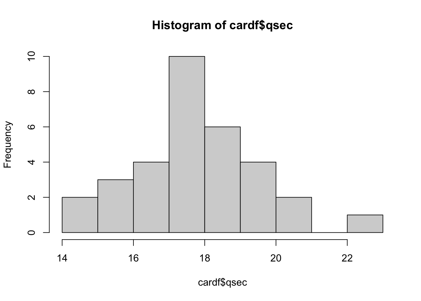
WOW! So pretty! look at you go.
Notice the title and x/y axis names. They aren’t pretty. We want clean titles to help with readibility. I won’t show you how to change these right now BUT you have the tools to figure this out for yourself. hint: ?hist
Think about what you can learn from the histogram vs. looking just at the numbers. Imagine if were looking at millions of data points! Plotting our data helps you get an idea of where the majority of values are. This is really important.
Create a new script and install the ‘RCPA3’ package.
Import the ‘world’ dataset from the RCPA3 package. I provide code for how to do that below:
#install.packages("RCPA3") Note: this is commented out because I have already installed it.
library(RCPA3)
world # The RCPA3 package has preinstalled datasets.
With the dataset, complete the following:
create a histogram for the percent of a country’s labor force that is in the military
add 2 variables together
subtract 1 variable from another
Before you begin, do some setup:
world2 <- world # create a new object to use for manipulation so that we do not alter the original dataWithout looking, could you tell me the following?
What does the ‘<-’ do?
What does the ‘$’ do?
Why do we need to visualize data?
Did you remember to add a heading to your R script?
Check your knowledge. Use the appropriate tools to figure out the answer to these questions. Consult the notes/readings/material if you do not know how to answer. “I don’t know” is not a sufficient answer.
What is the unit of analysis in the ‘mtcars’ dataset?
What is the unit of analysis in the ‘world’ dataset?
What is the mean of the variable ‘mpg’ in the ‘mtcars’ dataset?
What is our N for each dataset we looked at?
What do rows represent?
What do columns represent?
Homework 1 is now posted on Canvas! Make sure you follow the directions.
You should know who is in your group. Please contact them if you haven’t already. I provided everyone’s email, so check your email. I also assigned you to groups in Canvas.
You only have to turn in one copy - PLEASE WRITE THE NAME OF EVERYONE IN YOUR GROUP ON ALL DOCUMENTS TURNED IN!
Work together! Ask your group for help!
Use your notes, Youtube, peers, etc.
or scroll up and use all the notes I have given you!
All the resources I have given you should allow you to complete homework assignment with (relative) ease.
You will get errors! Double check your spelling, spacing, capitalization, etc.

😵💫
Please sit in your assigned groups! I will be giving you some time to work on your homework.
We have gone over quite a bit in these first few weeks. I want to spend this time to allow you to ask for clarification on anything we’ve gone over thus far. Any questions for me?
Why do we collect data?
What is a concept?
What is a variable?
What is operationalization?
What are you interested in? What is this thing you want to know about?
Are you interested in knowing about ideology? Democracy?
Cool! Now, how are going to measure these?
How will you collect data on this thing?
REMEMBER: Theory will guide your procedure in coding and data collection.
you need to define these concepts and defend your choices using theory.
Imagine someone asks, “why did you code Russia as a democracy?”
to defend yourself, you would explain how you define democracy and how Russia fits into your definition of democracy.
When we get data, we want to summarize key elements of individual variables.
Want to understand how the variable is distributed
How do we show the distribution? Histograms.
What is a typical value?
mean
median
mode (sortof)
How widely is the data dispersed around the typical value
range
standard deviation and variance
You only have to submit 1 assignment per group.
Every document turned in MUST have all members of the group listed.
Your script file should be organized.
IT MUST HAVE A HEADING INCLUDING THE FOLLOWING:
Names
Date
Title
I expect at least some comments adjacent to your code explaining what the code does.
Make sure you have both installed the packages needed and turned them on.
Divide the amount of work evenly. The homework is nicely divided to allow each individual to take one section.

I mean this whole thing is incredible. What I would do to be in the south of France dancing to this right now…You think I want to be here teaching you about variance?! JK I do <3 variance and standard deviation are very important.
P.S. - They are coming to Denver on January 27.
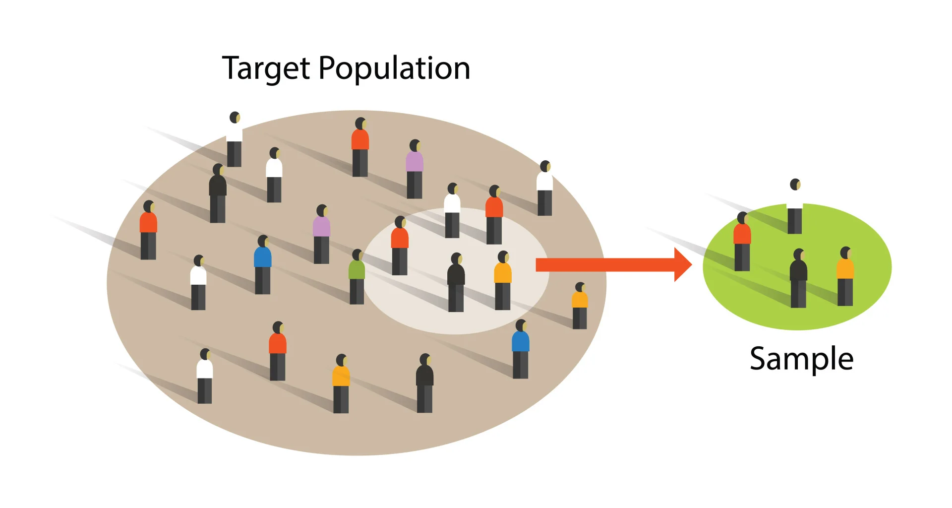
What is population?
What is a sample?
Why do we take samples? Why not just look at every person across the United States?
We are using data we have (sample) to tell us about data we don’t have (population!
Using a subset of the population can help us understand the population.
Samples can have biases!
There are different ways to sample.
how we sample is dependent on some factors but for the purposes of this class, we need need to ensure our sample is randomly collected.
not randomly sampling can bias our results.
There are different formulas for population variance/SD and sample variance/SD
What if I am looking at all 50 states (USA)? Would I use the population formula for variance and SD?
you will almost always use the sample formula.
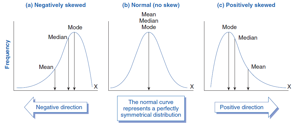
We want to know what a typical value is.
We talked before that the following help us figure this out:
mean
median
mode
We discussed in the lecture the pros and cons of these measures.
They are important though because they help us describe the data.
In general, we want our data to be normally distributed.
\[ \text{Variance} (s^2) = \frac{\sum_{i=1}^{n} (x_i - \bar{x})^2}{n-1} \]
Chill, chilllllll. Let’s go over what this all means.
Variance is a measure of SPREAD.
The average of the squared differences from the Mean.
Let’s walk through the formula step by step:
The \(\Sigma\) means to sum all the values together.
\((x_i - \bar{x})\)
in this part we are taking each observation and subtracting it by the mean (average).
Now lets add the square term. \((x_i - \bar{x})^2\)
Why do we square this?
Imagine a number line from 0 to 100. We have some dataset where the mean is 50. Now let’s say one of our observations is 38. 38-50 = -12. See what happens!? We have a negative number. All observations to the left of our mean are negative while all observations to the right of our mean are positive.
Thus we square to accommodate for these canceling out.
Now the \(n-1\)
N represents the number of observations.
Why are we subtracting it by 1?
If we were calculating the population variance, then we wouldn’t subtract by 1. However, we are pretty much never working with the population. We are always using some samples.
This part is not super intuitive. BUT, we are using the sample mean, NOT the population mean to calculate the variance.
We don’t know what the “true” population mean is. We have an estimate of it using our sample. Thus, there is some uncertainty around the sample mean (we don’t know if the sample mean is = to the population mean). To account for this uncertainty we add a -1 to our denominator.
By subtracting 1 from the denominator this makes the spread a little larger to account for that uncertainty. Think about what happens when we make our denominator smaller compared to if we don’t. Example:
\(\frac{16}{4-1}\) vs. \(\frac{16}{4}\)
\[ \text{Sample Standard Deviation} (s) = \sqrt{\frac{\sum_{i=1}^{n} (x_i - \bar{x})^2}{n-1}} \]
Standard deviation is literally the square root of variance.
Everything still means the same, we just square root it at the end.
WHY DO WE SQUARE ROOT?
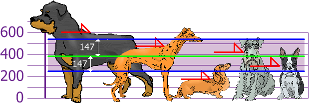
Why do we care about standard deviation?
see photo below:
This will be very important when we get to statistical inference!

Let’s work through an example together in R together.
StatQuest on Variance and SD. I would not be teaching you this if it weren’t for him.
Please get in contact with your new group.
It is due October 4th.
You MUST turn in the following:
a PDF of your responses
Please include the original question and your response.
Your R script.
This is where it gets a bit confusing.
Take your time. Watch some videos to reinforce this. This is not intuitive.
ASK QUESTIONS!

🦅 “Always searching, never perching” - incredible line. This is going to be my next instagram caption. 🦅
We can calculate how likely we are to get a sample result
When we sample, we introduce random error.
In essence, calculate how likely it is our sample is misleading.
Depends on:
law of large numbers
Central limit theorem
As the sample’s size approaches \(\infty\), sample mean will converge on the population mean
Sample must be random.
basically, bigger sample = better.
Very important!
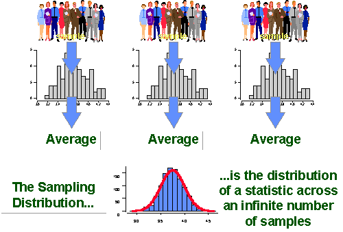
The distribution of a large number of sample means will be normally distributed around the population mean
Normal distribution: bell curve
Sampling distribution: distribution of possible samples
The sampling distribution gets tighter as the sample size increases.
This theorem is the critical math concept that allows us to do hypothesis testing.
Go back to the visual representation link from the central limit theorem section.
Imagine we took a bunch of samples.
Take the mean of each of those samples
now plot them like a histogram.
these are plotted as density plots.
\[ SE = \frac{SD}{\sqrt{n}} \]
the standard deviation of the sampling distribution
What is the difference between standard deviation and standard error?
Standard deviation quantifies the variation within a set of measurements. (singular)
Standard error quantifies the variation in the means from multiple sets of measurements. (multiple)
We (usually) only get one sample.
we want to know how likely our sample is given the sampling distribution.
we are trying to figure out where our sample is relative to other samples, assuming some null hypothesis.
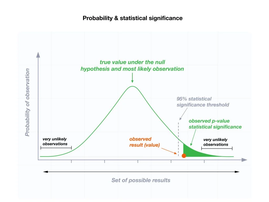
Basic idea: assuming some population mean, how probable is our sample?
Want to show that the data is unlikely given that assumption.
The p-value is extremely important and commonly misunderstood.
A p-value is the probability of observing a test statistic value equal to or more extreme than the value you computed if the null were true.
If we assume the null hypothesis is true, then we could draw the sampling distribution centered around zero (or whatever our value specified is). By specifing the null hypothesis we can invoke the central limit theorem.
The p-value is decided by the researcher. Convention typically sets the p-value at .10 and below. However, .10 is still not ideal, the lower the better.
Remember: we are using data we HAVE, to tell us about data we do NOT HAVE.
\(H_o\) : (null hypothesis) - I think the mean is not greater than x
\(H_A\) : (alternative hypothesis) - I think the mean is greater than x
For whatever variable you are interested in, report summary statistics on that variable. We want to know how our sample is distributed.
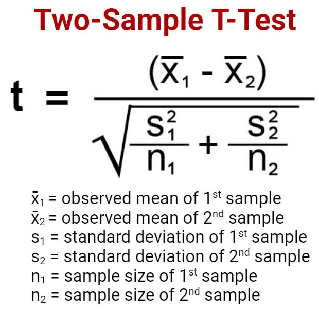
There are few different test statistics we can calculate. We will use a “Student’s” t-test. Fun fact, this statistical test was developed by the Guinness Beer Company. See statistics is important!
one sample t-Test formula:
\[ \frac{\bar{x} - \mu}{\frac{s}{\sqrt{n}}} \]
\(\bar{x}\) = observed mean of the sample
\(\mu\) = assumed mean
\(s\) = standard deviation
\(n\) = sample size
This is what R is doing under the hood when we run the t.test command. The t-score we compute from a t-test tells you how far the sample mean is from the hypothesized population mean in terms of the standard error.
We do NOT prove our hypothesis.
We can only do two things in the world of null hypothesis testing:
I reject the null hypothesis
I fail to reject the null hypothesis
I will show example code below. When we do this in R, we will get back a bunch of values.
We will get a “t value”.
“df” or degrees of freedom
p-value
As a researcher, I am interested in how people feel about Obama. I think to myself, hmm, I think the public likes Obama. But then I also remember, that a lot of people don’t like Obama. But, I think more people like Obama than not. I imagine that I ask everyone in the United States how I feel about Obama on a 0-100 scale. I can’t do this because I don’t know everyone and I don’t have enough money 😔. To figure this out, I take a sample, make a hypothesis, and test it!
\(H_o\) : The public’s average feeling towards Obama is \(\leq\) to 50
\(H_a\) : The public’s average feeling towards Obama is \(>\) than 50
Lucky for us, someone already took a sample. Wow, thank you RCPA3! Let’s call up that sample.
library(RCPA3)

nes <- nes #load nes dataset into environment
With our data loaded into R, let’s look at our sample feeling thermometer of Obama:
# calculate the mean of the 'ft.obama' variable in the nes dataset.
mean(nes$ft.obama, na.rm = TRUE) # the 'na.rm' is telling R to remove the NA values.
[1] 60.87802We now have a sample mean (\(\bar{x}\)) of 60.87802. Of our respondents, the average feeling towards Obama was 60.87802.
Now you might be thinking, 60.87802 > 50. Thus our alternative hypothesis is right. Case closed. Whoooooa, slow down buckaroo.
This is a SAMPLE. Maybe this sample is not that much different from the true population feeling thermometer toward Obama of 50. We need to know how likely it is we observed this sample given the population mean (the null hypothesis) was actually 50. But again, we don’t ever know the true population parameter. We assume the null hypothesis to be true. We are trying to see how likely it is for us to observe the value we got from our sample IF WE ASSUME THE POPULATION MEAN TO EQUAL 50.
We can use a test statistic to figure this out. Forgot what a t-test is? Scroll up.
t.test(nes$ft.obama, mu=50, alternative="greater") # do t-test of ft.obama, with hypothesis that the mean age is >50
    One Sample t-test

data:  nes$ft.obama
t = 26.727, df = 8164, p-value < 2.2e-16
alternative hypothesis: true mean is greater than 50
95 percent confidence interval:
 60.20847      Inf
sample estimates:
mean of x
 60.87802
Let’s go through what this means:
t = 26.727
this is our t-test score. Basically our sample that we observed is 26.727 standard errors away from our hypothesized mean of 50.
Remember this photo from earlier:
While this relates to standard deviations and is conceptually a bit different, it still should help.
Those numbers on the x-axis are standard errors. We can see the majority (99.7%) of all values lie within 3 standard errors of the mean.
df = 8164
degrees of freedom
after getting rid of the NA values we have 8165 observations
p-value < 2.2e-16
p-value definition: A p-value is the probability of observing a test statistic value equal to or more extreme than the value you computed if the null were true.
our p-value is in scientific notation
so it’s actually: \(0.00000000000000022\)
we know that we want p-values smaller than .10 (.05 and lower is better but I digress)
is this smaller than .10?
Interpretation:
we reject the null hypothesis
the public feeling thermometer towards Obama is \(\neq\) 50
Our sample mean is statistically greater than 50.
Remember! We never accept or “prove” our hypothesis.
Perhaps we have a binary or categorical variable. We want to see if the proportion we observed is statistically different from some value we specify. Everything is still the same but we will select a different variable and use different R code.
Let’s look at the variable ‘changed.names’. It asks whether people have changed names. I want to know how many people have changed names.
I am going to specify that more than 30% of people have changed names. Thus my hypothesis will look like the following:
\(H_0\) : \(p\leq .30\) the proportion is less than or equal to .30
\(H_A\): \(p>.30\) the proportion is greater than .30
summary(nes$changed.names) # find number in each category of whether people have changed names 1. Have changed name 2. Never changed name NA's
2672 5501 107 prop.test(2672, 2672+5501, p=.3, alternative="greater") # use number from summary command to conduct proportions test. Hypothesis is more than 30% of people have changed names
    1-sample proportions test with continuity correction

data:  2672 out of 2672 + 5501, null probability 0.3
X-squared = 28.097, df = 1, p-value = 5.768e-08
alternative hypothesis: true p is greater than 0.3
95 percent confidence interval:
 0.3183931 1.0000000
sample estimates:
        p
0.3269301
The prop.test argument is structured as such:
I am a strong believer that there is no “correct” way to teach this material. It helps to be exposed to different explanations. Here are some YouTube videos that helped me:
3Blue1Brown - Central Limit Theorem
zedstatistics - Standard Error
If you are thinking “Naur more statistics” then zedstatistics is your guy.
Statistics but with an Australian flair.
StatQuest with Josh Starmer - Central Limit Theorem

Do I need to say anymore?
Have not looked at it yet.
Hopefully went well?
Midterm is next week! Logistics are listed below:
There will be multiple choice.
There may be short answer response questions.
There will be an R portion.
You will have 2 hours to complete the test once you open it.
The test will be open for 24 hours.
ABSOLUTELY NO WORKING TOGETHER.
Midterm on October 16
For this week’s recitation, I am going to allow you to get into groups and collaborate on a study guide.
Some benchmark questions that may or may not be important for the midterm (but you should still know regardless!):
How do we find the mean?
How do we find the median?
How do we find the mode?
What do histograms tell us?
What is data?
What is the point of statistics?
What is the unit of analysis?
What is a concept?
True or False - observations are the columns in our data set.
What is a population?
What is a sample?
Why do we take samples?
Can you explain the central limit theory to me?
Why is the central limit theory important?
What is variance and how do we find it? What does it tell us?
What is standard deviation and how do we find it? What does it tell us?
What is standard error and how do we find it? What does it tell us?
I run a t-test and the R output shows a p-value of .12. What do I do?
Relatively speaking, do we usually want more observations or less in our data set?
I want to load the states data set into the R environment. I keep running this code but it keeps giving me an error!!!! UGH! What do I do?
states <- states hist(vep20.turnout)What is the definition of a p-value?
What is a null hypothesis? What is an alternative hypothesis?
Can we accept our hypothesis?
What is a confidence interval?
R gave me a bunch of code after I did a ‘t.test’. Can you help me understand what it means?
library(RCPA3)
# null hypothesis is feeling toward congress is equal to or greater than 50.
# alt hypothesis is feelign toward congress is less than 50
t.test(nes$ft.congress, mu = 50, alternative = "less")
    One Sample t-test

data:  nes$ft.congress
t = -22.32, df = 7354, p-value < 2.2e-16
alternative hypothesis: true mean is less than 50
95 percent confidence interval:
     -Inf 44.76362
sample estimates:
mean of x
 44.34697
Can you name a measure of central tendency? What do these values tell us?
I’m on a plane 10,000 feet in the air. Before jumping, I read a study about how there has been no randomized controlled trial of parachutes. Equipped with this knowledge, I dive head first out the door. Given what you now know about statistics, do we need theory? If so, why?
Do you know how to annotate your code?
What does ‘<-’ do?
What does ‘$’ do?
What is a function/command in R?
I have provided you with all the material possible for you to succeed on this midterm. I recommend you review the readings, lecture slides, your notes, and the material on this page. I want to remind you that this page is not intended to cover all the material. It is simply an additional resource to help guide you. If you are still fuzzy on material, come to my office hours next Tuesday. Alternatively, Professor Beard has office hours available. Additionally, I recommend YouTube videos on concepts you may still be struggling with.
Remember: You CAN do it.
I’ll see you on the other side of the midterm. 🫡

Midterm? What midterm? 💃🕺🪩
How was the midterm? Hard? Easy?
Anything you didn’t get?
Have you ever been interested in knowing if something causes another thing?
If you said YES then buckle in!
Data can help us answer these types of question.
We call our dependent variables ‘Y’
the variable we are interested in observing change in.
We (usually) put the dependent variable on the Y axis.
We call our independent variables ‘X’
It is a variable that we change aka the ‘treatment’.
We (usually) put the independent variable on the X axis
You’ve seen histograms
You’ve seen density plots
Now it’s time for scatter plots. (You all have seen this before at some point in your life.)
x <- mtcars$wt
y <- mtcars$mpg

# scatter plot code
plot(x, y, main = "Scatterplot Example",
     xlab = "Weight of Car", ylab = "Miles per Gallon ")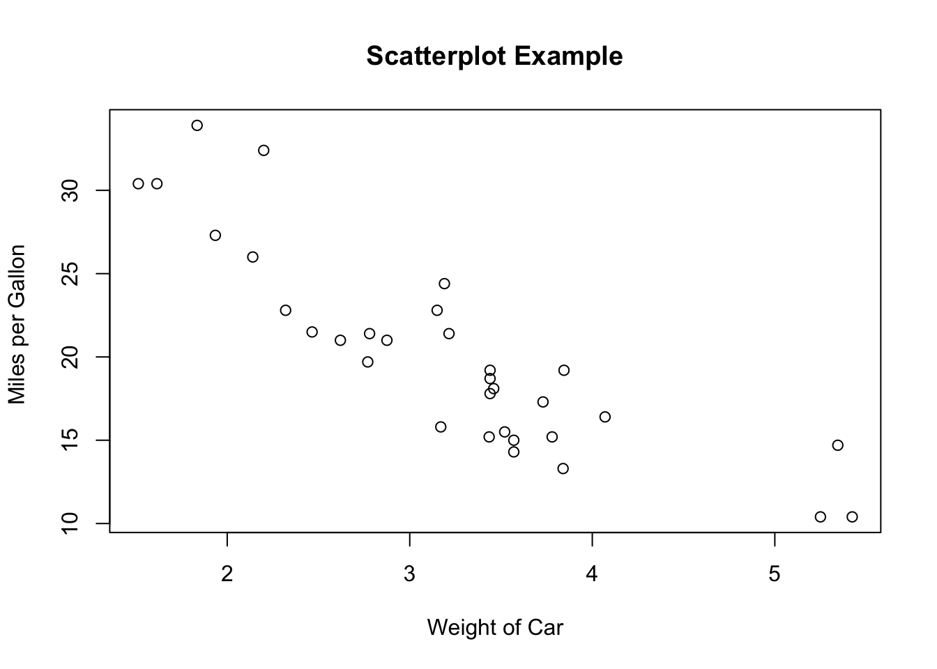
There is an example of a scatter plot.
Can we learn anything from this?
Regression is the big statistics dawg in town
Regression is a statistical tool we can use to see how much X causes change in Y.
Basically drawing a line in the middle of all the points.

I’m the main character today
We want to explain why things are the way they are
Independent Variables makes the Dependent Variable more likely.
Need theory!
Saying something causes another thing is HARD.
We are going to make lots of graphs because that helps us visualize the data.
Used if both variables are continuous
X-axis (horizontal line) = independent variable
Y-axis (vertical line) = dependent variable
Each point in a scatterplot is an observation.
library(RCPA3)

# using the world dataset, create a scatterplot of these two variables
plot(world$gdp.percap ~ world$trade.percent.gdp)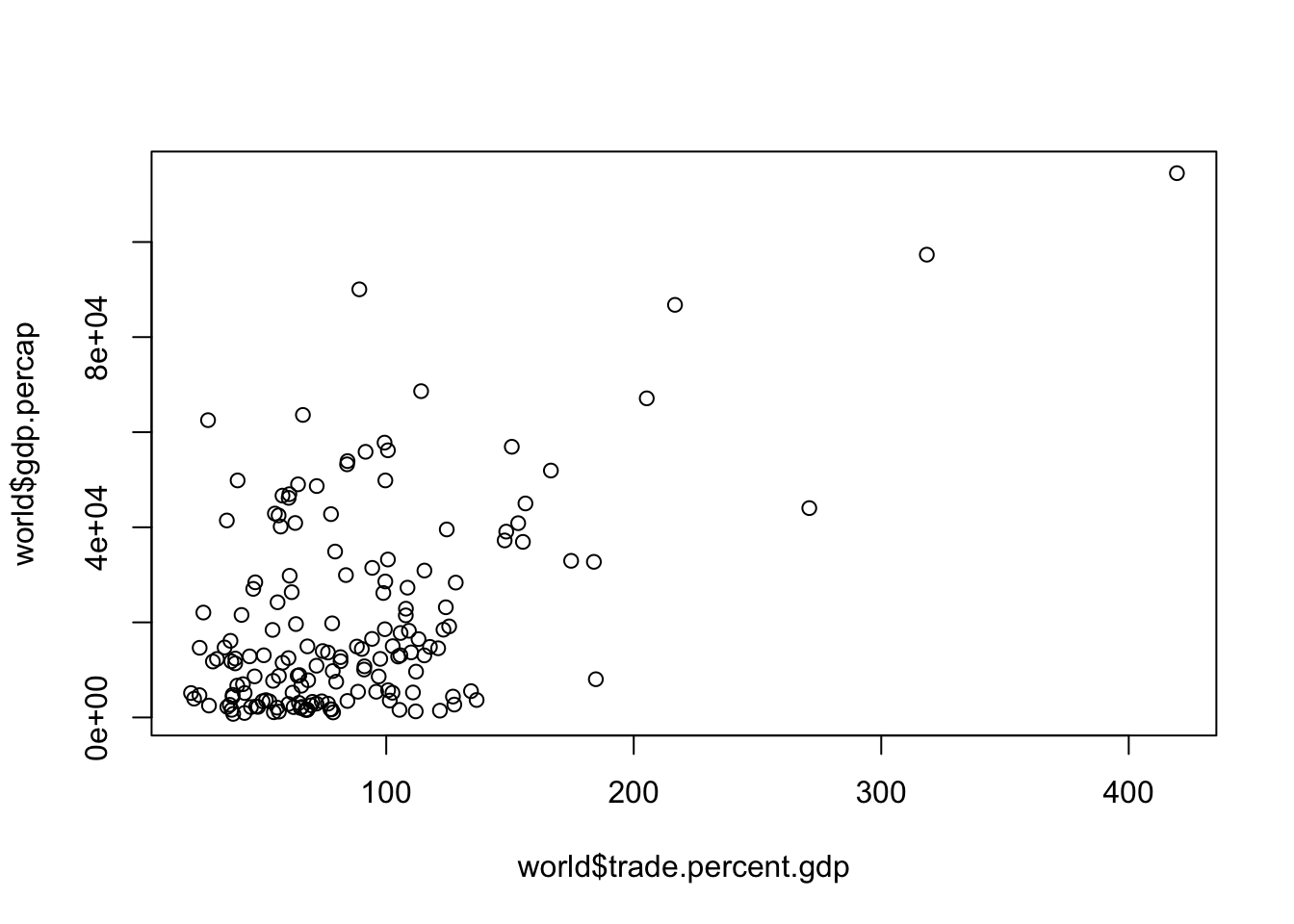
Each dot is a country (country is our unit of analysis)
We can change the scatterplot by adding arguments. These include titles, labels, changing how the points look, etc.
# Lets change some aspects of the scatterplot

# using the world dataset, create a scatterplot of these two variables
# Notice the arguments and what they do
plot(world$gdp.percap ~ world$trade.percent.gdp, main = "Trade v. GDP", xlab = "Trade as % GDP", ylab = "GDP per capita", pch = 14)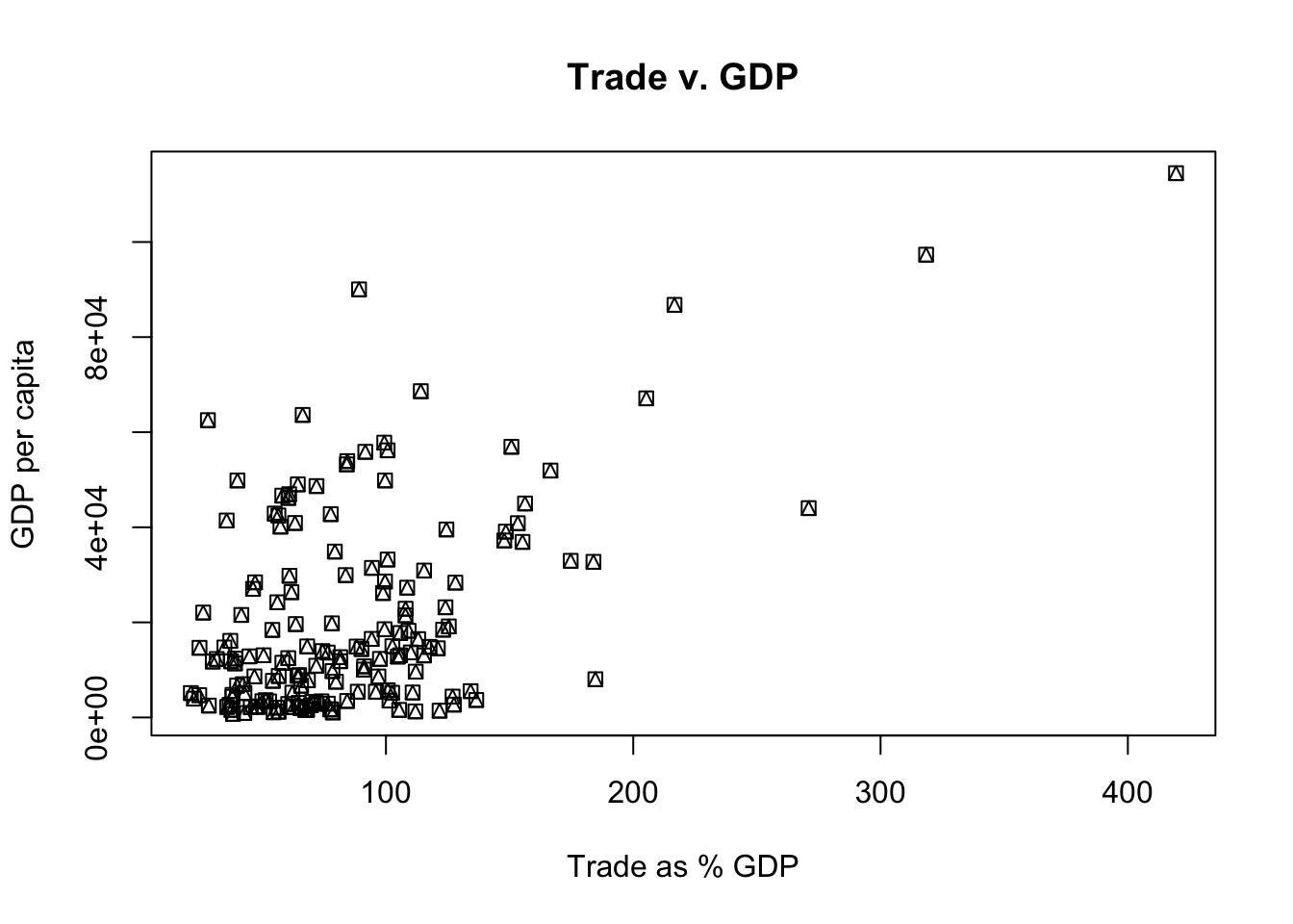
Useful to compare a continuous DV to a categorical/binary IV
Box: 1st (bottom - 25th percentile) and 3rd (top- 75th percentile) quartiles
Whiskers are range (max and min values)
# Boxplot of per capita GDP and whether Leader is Military Officer.
# using world dataset

# range=0 will include outliers in the whiskers
# so long as R knows IV is binary/categorical it will make a boxplot
# if R is not doing it then you need to check how R is reading it and change it accordingly
plot(world$gdp.percap~world$dpi.cemo, range=0, ylab = "GDP per capita", xlab = "Leader is Military Officer", main = "Boxplot Example") 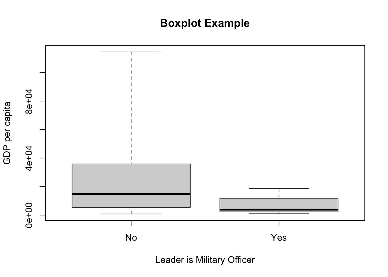
You did this earlier but it was a one sample t-test.
NOW, you are going to compare sample mean from one sample to the mean of another sample
are these two means statistically different?
Test how probable the observed difference between sample means would be if the population means were equal
Hypothesis: the mean of one group is greater/less than the mean of the other group
There is a formula associated with this. You don’t need to know it, R does it for you. However, I have posted it below if it helps you better understand what R is actually doing.
# two sample t-test example

# are the means different?
# is the "no" category greater than the "yes" category?
# same basic interpretation and procedure.
t.test(gdp.percap~dpi.cemo, data = world, alternative = "greater")
    Welch Two Sample t-test

data:  gdp.percap by dpi.cemo
t = 7.626, df = 152.65, p-value = 1.206e-12
alternative hypothesis: true difference in means between group No and group Yes is greater than 0
95 percent confidence interval:
 12859.44      Inf
sample estimates:
 mean in group No mean in group Yes
22893.698 6470.269 I am allowing you to form your own groups.
PUT YOUR NAMES ON EVERY DOCUMENT
You can do this solo (if you want)
4 people MAX

You know the vibes. 🎃
I have graded all midterms.
Should be released soon.
Correlation does not equal causation!
We interpret correlation from -1 to 1.
-1 represents a perfectly negative correlation
This will almost never happen
1 represents a perfectly positive correlation
Correlation tell us the direction and strength of a linear relationship between two variables.
If you were to get a correlation of zero. What would that look like?
Let’s go over a quick example from the car data
cor(mtcars$mpg, mtcars$wt)[1] -0.8676594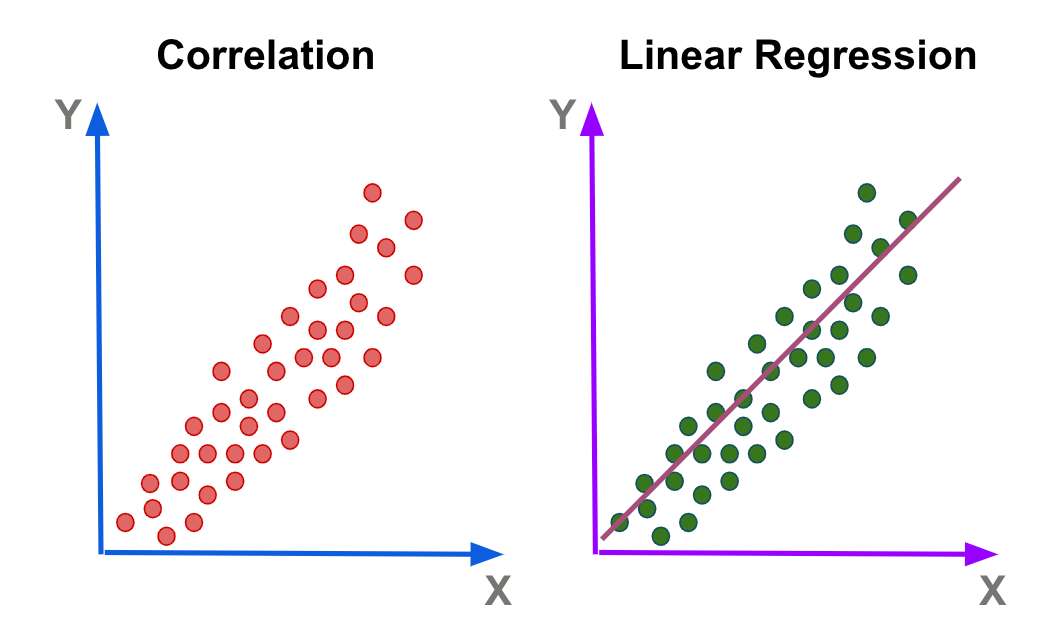
Here is a great website of spurious correlations
This is why theory matters!
- correlation just quantifies the covariance of two variables into an output between -1 and 1.Regression tells us how one variable impacts the other.
Also called Ordinary Least Squares (OLS)
How much X causes variation in Y.
What are we doing in regression
we are drawing a line that minimizing the sum of squares.
literally drawing a line in the middle of all the observations
How do we know what line to draw?
Error…what is it?
typically represented in mathematical notation as \(\epsilon\) (epsilon).
it is the variation in our dependent variable we cannot explain by our independent variable.
\(y_i - \hat{y}_i\)
Let’s go over this real quick. Don’t worry if you are still fuzzy. We are going to keep going over this in later weeks.
# regression
# DV: mpg
# IV: wt (weight)
summary(lm(mtcars$mpg~mtcars$wt))
Call:
lm(formula = mtcars$mpg ~ mtcars$wt)

Residuals:
    Min      1Q  Median      3Q     Max
-4.5432 -2.3647 -0.1252  1.4096  6.8727

Coefficients:
            Estimate Std. Error t value Pr(>|t|)
(Intercept)  37.2851     1.8776  19.858  < 2e-16 ***
mtcars$wt    -5.3445     0.5591  -9.559 1.29e-10 ***
---
Signif. codes:  0 '***' 0.001 '**' 0.01 '*' 0.05 '.' 0.1 ' ' 1

Residual standard error: 3.046 on 30 degrees of freedom
Multiple R-squared:  0.7528,    Adjusted R-squared:  0.7446
F-statistic: 91.38 on 1 and 30 DF,  p-value: 1.294e-10
The old me is dead and gone but that new me will be alright 🧑👈🙏💪
minimize the sum of squared residuals
What is a residual?
vertical distance from point to line
\(y_i - \hat{y}_i\)
note: a residual might also be called “error”.
The error/residual is how much our line of best fit DOES NOT explain.
We are going to minimize the error across ALL OBSERVATIONS.
thus we are drawing a line that perfectly does that
of course, we can draw an infinite number of lines. So how do we know what line is best?
there is a formula that you do not need to know:
Let’s first make a scatterplot:
library(RCPA3)
plot(states$cigarettes ~ states$cig.tax, main = "cigarette taxes and smoking", xlab = "cigarette tax/pack", ylab = "Mean num. of packs bimonthly")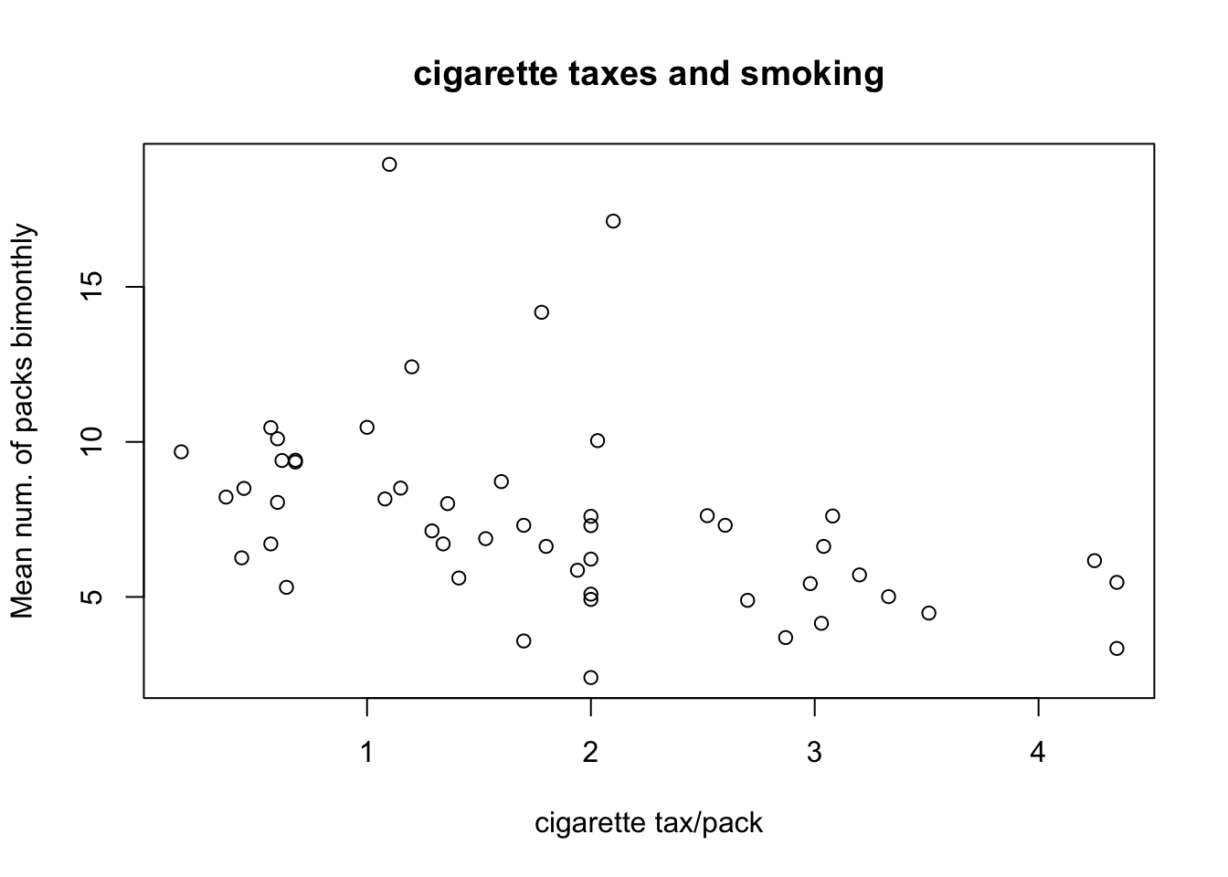
Let’s run a regression now.
Dependent variable: cigarette consumption by state
Independent variable: cigarette tax by state
model <- lm(states$cigarettes ~ states$cig.tax) #run a bivariate regression and call it 'model'
summary(model) # show the results of the regression model
Call:
lm(formula = states$cigarettes ~ states$cig.tax)
Residuals:
Min 1Q Median 3Q Max
-4.9640 -1.3838 -0.3718 0.8209 10.4901
Coefficients:
Estimate Std. Error t value Pr(>|t|)
(Intercept) 9.7994 0.8065 12.151 2.97e-16 ***
states$cig.tax -1.2177 0.3798 -3.206 0.00239 **
---
Signif. codes: 0 '***' 0.001 '**' 0.01 '*' 0.05 '.' 0.1 ' ' 1
Residual standard error: 2.91 on 48 degrees of freedom
Multiple R-squared: 0.1764, Adjusted R-squared: 0.1592
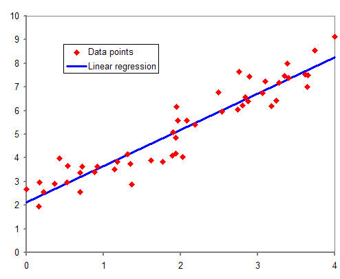
F-statistic: 10.28 on 1 and 48 DF, p-value: 0.002394Let’s add the regression line to the scatterplot.
plot(states$cigarettes ~ states$cig.tax, main = "cigarette taxes and smoking", xlab = "cigarette tax/pack", ylab = "Mean num. of packs bimonthly")
abline(model, col = "red") # adds a line to plot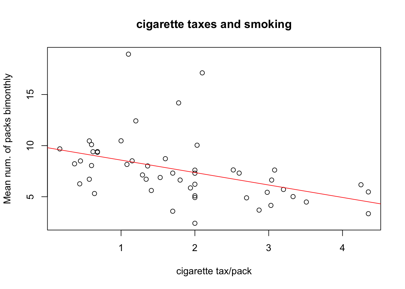
The code above is a little messy. We can use a new package called ‘ggplot2’ to create a plot. We can load the ‘tidyverse’ package which contains ggplot2.
This might look a little more confusing but take the time to dig in and I think you can start to see why this is a bit better. Additionally, ggplot2 has an insane amount of customization. This package allows you to basically make any plot you can think of.
library(tidyverse)Warning: package 'purrr' was built under R version 4.3.3── Attaching core tidyverse packages ──────────────────────── tidyverse 2.0.0 ──
✔ dplyr 1.1.4 ✔ readr 2.1.5
✔ forcats 1.0.0 ✔ stringr 1.5.1
✔ ggplot2 3.5.1 ✔ tibble 3.2.1
✔ lubridate 1.9.2 ✔ tidyr 1.3.1
✔ purrr 1.0.4
── Conflicts ────────────────────────────────────────── tidyverse_conflicts() ──
✖ dplyr::filter() masks stats::filter()
✖ dplyr::lag() masks stats::lag()
ℹ Use the conflicted package (<http://conflicted.r-lib.org/>) to force all conflicts to become errors# ggplot version
ggplot(states, aes(x = cig.tax, y = cigarettes)) +
geom_point() + # Scatter plot of the data
geom_smooth(method = "lm", se = TRUE, color = "red") + # Add linear regression line
labs(
title = "Cigarette Taxes and Smoking",
x = "Cigarette Tax/Pack",
y = "Mean Num. of Packs Bimonthly")`geom_smooth()` using formula = 'y ~ x'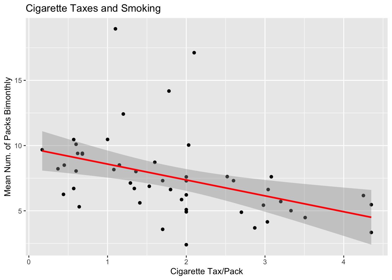
See! Doesn’t that look so much better? Do you know what that band is around the line?
Groups are up to you.
Due next week.

This room is our sanctuary for statistics. There is no pain when we learn statistics
WE WILL HAVE RECITATION NEXT WEEK (BEFORE THANKSGIVING BREAK)!
I finished grading homework 3
It seems we are struggling with interpretation of our results.
You should always say whether you reject or fail to reject the null hypothesis!
What area do you feel you need more help with?
We loosely went over this earlier but I wanted to circle back.
When we do regression we still specify our null and alternative hypothesis.
These will look like the following:
Null Hypothesis \(\beta = 0\)
Alternative Hypothesis \(\beta \neq 0\)
If our coefficient is statistically different, that means our (coefficient/slope) is statistically different from zero!
Same thing as bivariate regression but with more variables!
Past 3 variables we can’t really visualize this with all the dimensions. It will hurt your brain! (So, don’t do it!)
Multivariate regression allows us to “control” for other variables.
By controlling for other variables, we can isolate the effect our variable we are interested in.
library(RCPA3)
model_bivariate <- lm(cigarettes ~ cig.tax, data = states) # create regression and assign to object
summary(model_bivariate) # print summary statistics for regression model
Call:
lm(formula = cigarettes ~ cig.tax, data = states)

Residuals:
    Min      1Q  Median      3Q     Max
-4.9640 -1.3838 -0.3718  0.8209 10.4901

Coefficients:
            Estimate Std. Error t value Pr(>|t|)
(Intercept)   9.7994     0.8065  12.151 2.97e-16 ***
cig.tax      -1.2177     0.3798  -3.206  0.00239 **
---
Signif. codes:  0 '***' 0.001 '**' 0.01 '*' 0.05 '.' 0.1 ' ' 1

Residual standard error: 2.91 on 48 degrees of freedom
Multiple R-squared:  0.1764,    Adjusted R-squared:  0.1592
F-statistic: 10.28 on 1 and 48 DF, p-value: 0.002394before we run the multivariate regression, we need to think about what other variables may influence cigarette use.
What variables influence cigarette use? This is why theory is important!
I can think of a few from the ‘states’ dataset (there are more):
age (“median.age”)
education (“ba.or.more”)
income (“prcapinc”)
model_multivariate <- lm(cigarettes ~ cig.tax + median.age + ba.or.more + prcapinc, data = states) # create regression and assign to object
summary(model_multivariate) # print summary statistics for regression model
Call:
lm(formula = cigarettes ~ cig.tax + median.age + ba.or.more +
    prcapinc, data = states)

Residuals:
    Min      1Q  Median      3Q     Max
-4.3902 -0.8428 -0.3169  0.4261  9.3813

Coefficients:
              Estimate Std. Error t value Pr(>|t|)
(Intercept) -1.200e+01  6.705e+00  -1.790 0.080175 .
cig.tax     -1.364e+00  4.218e-01  -3.233 0.002293 **
median.age   6.038e-01  1.624e-01   3.718 0.000553 ***
ba.or.more  -2.235e-01  1.119e-01  -1.997 0.051898 .
prcapinc     1.809e-04  1.397e-04   1.295 0.201870
---
Signif. codes:  0 '***' 0.001 '**' 0.01 '*' 0.05 '.' 0.1 ' ' 1

Residual standard error: 2.495 on 45 degrees of freedom
Multiple R-squared:  0.4325,    Adjusted R-squared:  0.3821
F-statistic: 8.574 on 4 and 45 DF,  p-value: 3.125e-05
Scroll up and compare the results to the bivariate result. What do you notice?
Do you remember how to interpret this?
Some of you may be a bit confused about the first part of the homework
The point of this exercise is to find a line of best fit.
We want to find a line that minimizes the residuals
but how do we know what the residuals are without the line of best fit?!

What are you still doing here? Go HOME! 🪩
Anyone have strong feelings about Thanksgiving food?
I love stuffing and mashed potatoes (shoutout carbs)
This year we are mixing it up. Smoking a brisket and some pork.
Potentially unlimited variables:
Independent variable/s (IV)
Dependent variable (DV)
Control variables
Estimates effects of IV/s on DV
Not as easy to interpret
Can do a better job of explaining variation (Adjusted R2)
Might do a better job of arguing causation
We will get \(\beta\) coefficients (remember \(\beta\) is the slope) for each of our variable. This is the effect of that IV on the DV, holding other variables constant. Though we get a \(\beta\) coefficient for each variable, we also get a t-test and respective p-value for each output.
“for every one unit change in X, we observe a ____ change in Y.
“for every one unit change in X, we observe a ____ change in Y, all else equal.”
“the expected change in Y for [category X] is ____, when compared to [reference category].”
This one is not as clean. These don’t need to be written exactly like this but you need to get the same message across to the reader when you write this.
model_multivariate <- lm(cigarettes ~ cig.tax + median.age + ba.or.more + prcapinc, data = states) # create regression and assign to object
summary(model_multivariate) # print summary statistics for regression model
Call:
lm(formula = cigarettes ~ cig.tax + median.age + ba.or.more +
    prcapinc, data = states)

Residuals:
    Min      1Q  Median      3Q     Max
-4.3902 -0.8428 -0.3169  0.4261  9.3813

Coefficients:
              Estimate Std. Error t value Pr(>|t|)
(Intercept) -1.200e+01  6.705e+00  -1.790 0.080175 .
cig.tax     -1.364e+00  4.218e-01  -3.233 0.002293 **
median.age   6.038e-01  1.624e-01   3.718 0.000553 ***
ba.or.more  -2.235e-01  1.119e-01  -1.997 0.051898 .
prcapinc     1.809e-04  1.397e-04   1.295 0.201870
---
Signif. codes:  0 '***' 0.001 '**' 0.01 '*' 0.05 '.' 0.1 ' ' 1

Residual standard error: 2.495 on 45 degrees of freedom
Multiple R-squared:  0.4325,    Adjusted R-squared:  0.3821
F-statistic: 8.574 on 4 and 45 DF, p-value: 3.125e-05Make sure you are evaluating the other columns before answering!
\[ n-k-1 \]
This is formula for Degrees of Freedom
Where:
\(n\) = the number of observations
\(k\) = the number of parameters estimating (the number of independent variables)
\(-1\) = literally just minus 1. Not entirely sure why we do this.
Degrees of freedom relate to how much information we have available to estimate something.
I like to use Anand Sokhey’s example of pixels and a photograph.
the more pixels you have in an image, the clearer it is (more observations)
the less pixels you have, the less information you have, and the harder it is to figure out what the image is (less observations)
Same command in R
Slightly different interpretation:
Yes = 1; No = 0 (the intercept)
Command:

Trickier!
You’re comparing the coefficients to each other since the units are meaningless.
For example, what would a 1-unit increase in blue eye color mean???
Instead, you choose one of the independent variables as a reference category and base your interpretation off of a comparison to that category.
“Brown-eyed students score 0.3% higher on the midterm relative to blue-eyed students.”
I made this up.
Command is the same; be sure to list your desired ref category as IV1
Recall a binary IV is coded as 0 or 1. When you run a regression with this type of variable, R will not include the reference category (which will be 0). There is a mathematical reason for this called perfect mulit-collinearity.
Perfect Multi-Collinearity: is when one IV perfectly explains the other.
example: you have a variable coded as the following:
0 = Democrat
1 = Republican
| Trump_ft (feeling therm) | Democrat | Republican |
|---|---|---|
| 49 | 1 | 0 |
| 21 | 1 | 0 |
| 64 | 1 | 0 |
| 83 | 0 | 1 |
imagine your dataframe looked like that.
if you were to include both the Democrat and Republican variable in your regression, you would run into some issues.
Why?
Your ‘Democrat’ variable perfectly predicts the ‘Republican’ variable.
To avoid this, we have a reference category. If we were to run a regression, Democrats would not be included in the output table. We would get the coefficient for Republican feelings toward Trump.
# create a data frame
df <- data.frame(
  trump_ft = c(49, 21, 64, 83),
  Democrat = c(1, 1, 1, 0),
  Republican = c(0, 0, 0, 1)
)

# regression
summary(lm(trump_ft~Democrat + Republican, data = df))
Call:
lm(formula = trump_ft ~ Democrat + Republican, data = df)

Residuals:
         1          2          3          4
 4.333e+00 -2.367e+01  1.933e+01  5.107e-15

Coefficients: (1 not defined because of singularities)
            Estimate Std. Error t value Pr(>|t|)
(Intercept)    83.00      21.83   3.803   0.0627 .
Democrat      -38.33      25.20  -1.521   0.2676
Republican        NA         NA      NA       NA
---
Signif. codes:  0 '***' 0.001 '**' 0.01 '*' 0.05 '.' 0.1 ' ' 1

Residual standard error: 21.83 on 2 degrees of freedom
Multiple R-squared:  0.5364,    Adjusted R-squared:  0.3045
F-statistic: 2.314 on 1 and 2 DF,  p-value: 0.2676
notice the output says “Coefficients: (1 not defined because of singularities)”
Punchline: think about how the IVs you choose might be related to each other. It is fine if they are related but it becomes a big problem when they perfectly relate to each other.
We use interactions when we have a conditional hypothesis. Example:
Don’t worry about this right now. We will go over this more after the break.
install.packages("stargazer")
library(stargazer)
Stargazer is a very useful package. Think about what you know so far from the regression outputs we have been looking at. Why do you think this package is called stargazer?
Stargazer makes our outputs pretty and easier to read. They also allow us to compare across different models.
Let’s use an example. First, let’s create some regression models:
library(RCPA3)
library(stargazer)
Please cite as: Hlavac, Marek (2022). stargazer: Well-Formatted Regression and Summary Statistics Tables. R package version 5.2.3. https://CRAN.R-project.org/package=stargazer model0 <- lm(trade.percent.gdp~tariff.rate, data=world)
model1 <- lm(trade.percent.gdp~tariff.rate + eiu.democ.bin + eu + religion, data=world) #
model2 <- lm(trade.percent.gdp~ eiu.democ.bin*tariff.rate + eu, data=world)
stargazer(model0, model1, model2 , type="text", report="vcs*",star.char = c("+","*","**","***"), star.cutoffs=c(.1,.05,.01,.001), notes="+p<0.1,*p<0.05,**p<0.01,***p<0.001", notes.append=FALSE)
==================================================================================================
                                                      Dependent variable:
                             ---------------------------------------------------------------------
                                                       trade.percent.gdp
                                       (1)                    (2)                    (3)
--------------------------------------------------------------------------------------------------
tariff.rate                          -3.941                  -2.499                 -2.121
                                   (0.892)***               (1.048)*               (1.229)+

eiu.democ.binYes                                             -4.306                 1.992
                                                            (10.187)               (18.394)

euNo                                                        -49.064                -44.878
                                                          (12.334)***            (12.980)***

religionCatholic                                            -38.107
                                                           (16.105)*

religionMuslim                                              -36.070
                                                           (16.327)*

religionNA                                                  -94.694
                                                           (49.748)+

religionOrthodox Christian                                  -32.184
                                                           (19.117)+

religionOther                                               -36.405
                                                           (20.233)+

religionOther Christian                                     -37.298
                                                           (17.024)*

eiu.democ.binYes:tariff.rate                                                        -0.917
                                                                                   (2.217)

Constant                             115.340                181.810                140.336
                                   (7.664)***             (21.578)***            (18.080)***

--------------------------------------------------------------------------------------------------
Observations                           159                    159                    159
R2                                    0.111                  0.235                  0.196
Adjusted R2                           0.105                  0.189                  0.175
Residual Std. Error             49.574 (df = 157)      47.187 (df = 149)      47.604 (df = 154)
F Statistic                  19.533*** (df = 1; 157) 5.094*** (df = 9; 149) 9.362*** (df = 4; 154)
==================================================================================================
Note:                                                           +p<0.1,*p<0.05,**p<0.01,***p<0.001
sjPlot is another package to help visualize results.
I’ve showed you ‘ggplot2’ which is another package created for the same task.
There are many different ways to visualize this stuff. This is just to expand your pallet and learn about all the options you have available!
# make sure you have the sjPlot package installed first!
# we are using the 'model2' from the previous code chunk
library(sjPlot)
Warning: package 'sjPlot' was built under R version 4.3.3Install package "strengejacke" from GitHub (`devtools::install_github("strengejacke/strengejacke")`) to load all sj-packages at once!plot_model(model2, type="pred", term=c("tariff.rate", "eiu.democ.bin"))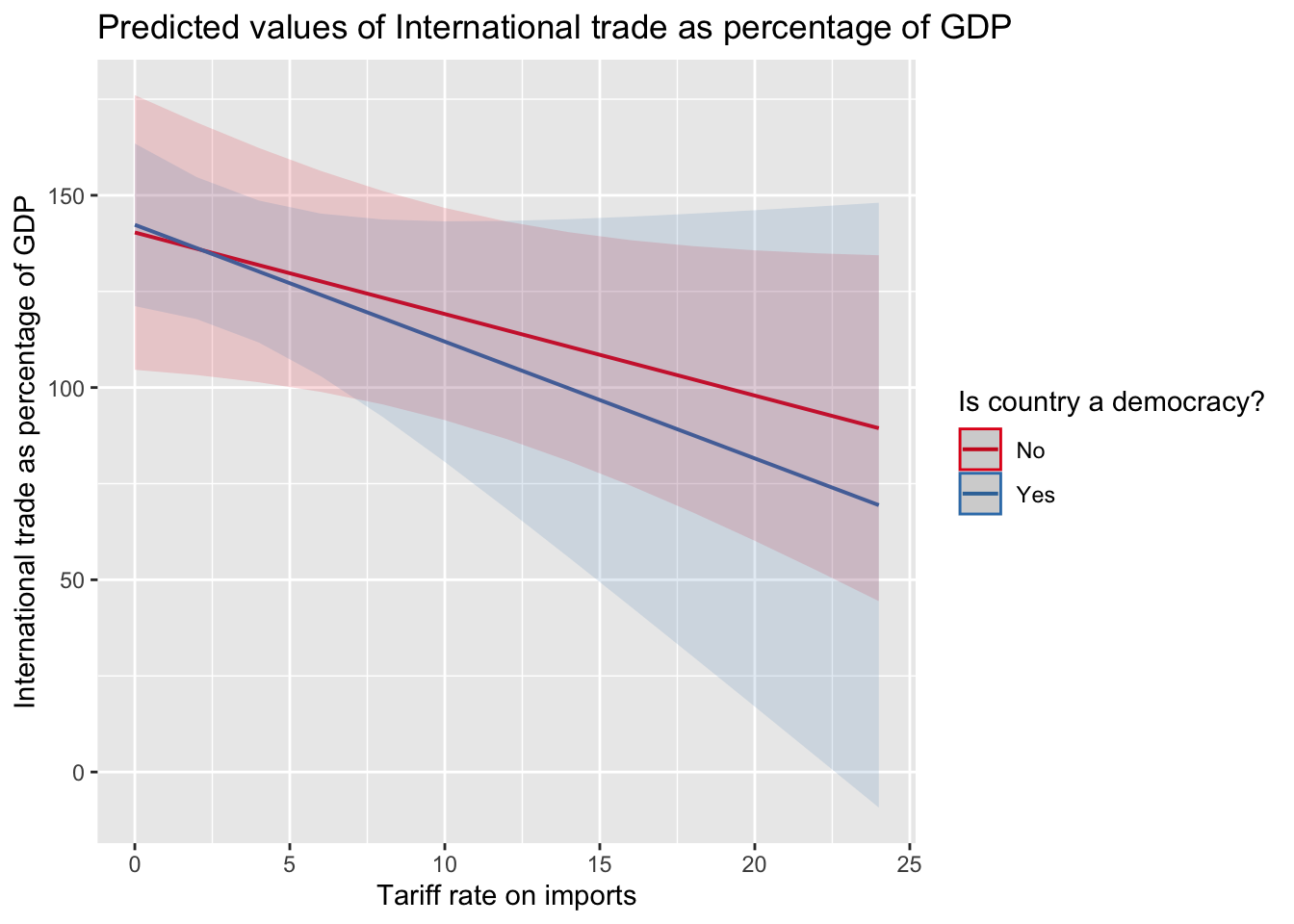
While we observe a general decrease in trade as tariffs go up, we cannot statistically differentiate the effect of being a democracy on this relationship. We can tell because the confidence intervals overlap. We will go over this more after break.

We are SO BACK (literally).
Make sure I haven’t made any mistakes.
If I did, email me explaining the issue.
Haven’t put it together yet.
Will likely focus on more recent material but anything is possible.
We will do review next week. Let me know if there is any specific material you want me to go over.
We use interactions for conditional hypothesis.
Example: X causes Y, only if Z is active. The effect of X on Y depends on the level of Z.
When interactions are dichotomous or categorical, interpretation is relatively easy. When the interaction includes a continuous variable, interpretation from the table becomes difficult.
In a regression with interactions, we include all constitutive terms.
Wrong: Turnout = Age + Age*Race
Correct: Turnout = Age + Race + Age*Race
Let’s look at the example from lecture. We want to know if the effect of tariff rates on trade is conditional on whether the country is democratic or not.
library(RCPA3)
# note R will include the constitutive terms automatically.
model_int <- lm(trade.percent.gdp~ eiu.democ.bin*tariff.rate + eu, data=world)
summary(model_int)
Call:
lm(formula = trade.percent.gdp ~ eiu.democ.bin * tariff.rate +
    eu, data = world)

Residuals:
    Min      1Q  Median      3Q     Max
-76.704 -28.764  -8.067  21.700 286.256

Coefficients:
                             Estimate Std. Error t value Pr(>|t|)
(Intercept)                  140.3363    18.0803   7.762 1.08e-12 ***
eiu.democ.binYes               1.9921    18.3940   0.108 0.913896
tariff.rate                   -2.1211     1.2292  -1.726 0.086429 .
euNo                         -44.8779    12.9799  -3.457 0.000705 ***
eiu.democ.binYes:tariff.rate  -0.9169     2.2171  -0.414 0.679784
---
Signif. codes:  0 '***' 0.001 '**' 0.01 '*' 0.05 '.' 0.1 ' ' 1

Residual standard error: 47.6 on 154 degrees of freedom
  (10 observations deleted due to missingness)
Multiple R-squared:  0.1956,    Adjusted R-squared:  0.1747
F-statistic: 9.362 on 4 and 154 DF, p-value: 8.456e-07library(sjPlot)
plot_model(model_int, type="pred", term=c("tariff.rate", "eiu.democ.bin")) #plot interaction from model2, with different lines for eiu.democ.bin
model_simple <- lm(trade.percent.gdp~ tariff.rate + eu + eiu.democ.bin, data=world)
plot_model(model_simple, type="pred", term=c("tariff.rate"))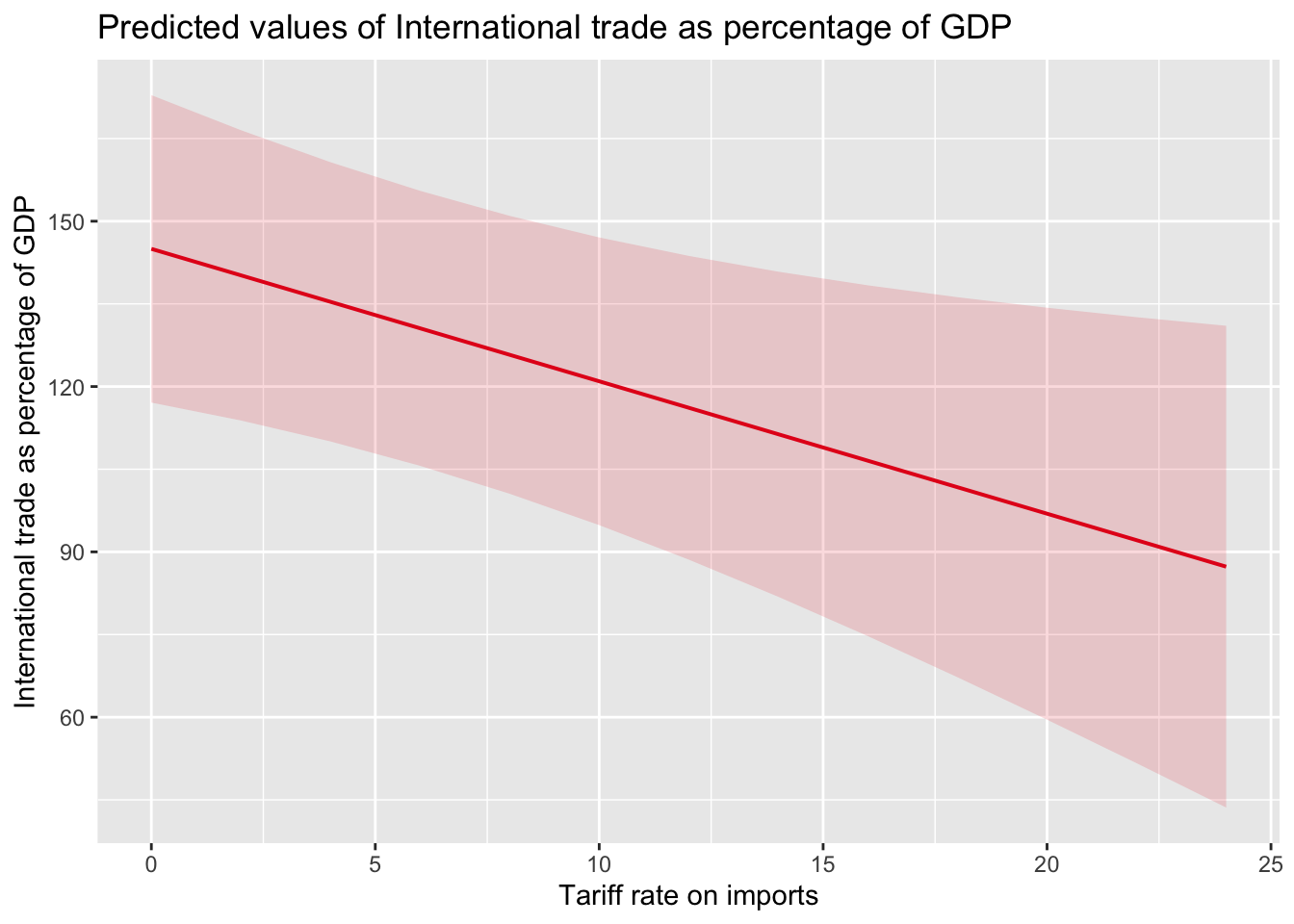
Spend the rest of class working on Homework 5!
It is due soon!

FYI - I was successful in getting their concert tickets at Red Rocks. 😎
Justice was my #1 wrapped spotify artist. Low key like their biggest fan.
Also, this is our last class so this felt like a fitting song. Literally, THE END.
Thank you all for a fun semester! This was my first time teaching statistics. Hopefully, I made it (somewhat) digestible for you.
Final will take place on December 17.
24 hour window. 12:01 AM to 11:59 PM
You will have 2.5 hours to complete once started.
Will be online.
NO EXTENSIONS OR MAKE-UP DATES.
Similar format to midterm. Expect ‘select all that apply’ questions and a coding portion. Will need to upload R script.
Likely include questions across the semester but will focus on latter material.
Remember that this material builds upon each other!
No AI or working with anyone else.
I provide the answer beneath each question. It is hidden in the foldable section under each question.
DON’T LOOK AT ANSWER UNTIL YOU HAVE ANSWERED THE QUESTION.
These are topics I think are important for you to know. It is not comprehensive and you should consult other material (textbook, lecture, homework, etc.) when studying.
Use this to guide you study but do not rely on it.
What is the point of statistics?
"To use data we have to tell us about data we don't have!"I want to know how good students are doing in PSCI 2075. I sample only students in in my recitations. Is this an issue? Why?
"Sampling only students in my recitation to make inferences about all students in PSCI 2075 would be problematic because I would have a selection bias. My sample is not a random sample. Students may differ in their grades because of different TAs. By only looking at my students, I fail to control for other factors (like having a different TA) on a student's grade. Thus the sample is not representative of the population of interest."Are random samples good? Why or why not?
"They are good. I won't tell you why here. You should go read about it from the book or earlier material/lecture notes to answer this question."There are no randomized controlled experiments that show the effectiveness of parachutes. Should I jump out of this airplane without a parachute?
"Do you really need to see the answer to this?"True or False: Research questions must be falsifiable.
"True."What is an ordinal variable?
"A categorical variable that has a hierarchy between each category."The mean, median, and mode are all measures of what?
"Central tendency"What is the difference between variance and standard deviation?
"Standard deviation is the square root of variance."
"Variance is about the spread of the data; standard deviation standardizes the spread into one number."
What axis does the dependent variable go on? What axis does the independent variable go on?
"Dependent variable goes on the Y axis."
"Independent variable goes on the X axis."Jon wants to compare his students performance to Stone’s students performance. Jon has two variables. Using the description of the variables below, what plot should Jon create?
stone_student_grades: a continuous variable containing the grade percentage of each of his students.
jon_student_grades: a continuous variable containing the grade percentage of each of his students.
"Because these are both continuous variables, Jon should create a scatterplot."Paul “Lisan Al-Gaib” Atreides wants to know the concentration of spice (melange) between the cities of Arrakeen and Sietch Tabr. With the information below, how should the Lisan Al-Gaib plot these variables?
“city” is a binary variable
“spice_concentration” is a continuous variable
"Because one variable is binary and the other is a continous, the Lisan Al-Gaib should create a boxplot."


"~the spice must flow~"Can you explain the Central Limit Theorem to someone? No like, literally, can you? Turn to a friend, neighbor, or call up your mom and see if you can explain it in a way that they would understand.
"Return to earlier weeks to review the concept. The central limit theorem is important! It is the mechanism that allows us to do hypothesis testing! Think about what the central limit theorem is and why it might be related to null hypothesis testing."What does the Central Limit Theorem allow us to do?
"The central limit theorem allows us to do hypothesis testing!"What is the purpose of hypothesis testing?
"To use data we have to tell us about data we don't have! We use it to make inferences with our sample data. Is this a real relationship or is this just a relationship I observe due to chance? Hypothesis testing helps us understand this connection."What is the purpose of having a null hypothesis?
"It provides a baseline to compare to. The null hypothesis represents the assumption of no relationship in the population. If the null were true, how likely are we to observe the sample we got? If it is unlikely for us to observe the sample we got (which we determine using the test stat and p-value) then it is improbable that we observed the sample to do chance."What is a p-value?
"A p-value is the probability of observing a test statistic value equal to or more extreme than the value you computed if the null were true."What is a confidence interval?
"The range of true values that would give our sample (or something
further away) at least some portion of the time"

"A confidence interval is the mean of your estimate plus and minus the variation in that estimate. This is the range of values you expect your estimate to fall between if you redo your test, within a certain level of confidence."A regression has multiplication between two variables in it. What is that called?
"Interaction"How many independent variables are included in a bivariate regression?
"One variable."What is the null hypothesis in Regression?
"beta = 0"Why do we add control variables?
"A control variable is an independent variable that you believe does not have a causal effect upon the dependent variable, but would potentially bias your results by excluding from your model (i.e. age, level of education, GDP per capita, population, etc.)" I estimate a bivariate model between cigarette consumption and cigarette taxes. I don’t include age in my regression equation even though I think it is a theoretically important factor on the consumption of cigarettes by state. What type of bias is this an example of?
"This is considered an ommitted variable bias."What is a residual?
"The residual is the difference between our observed value and the predicted value (the regression line.) Note: the residual may also sometimes be called the error."What does the line of best (regression line) do?
"It minimizes the sum of squares. Hence the name OLS - Ordinary Least Squares"Can we do a regression with a binary independent variable?
"Yes! When we have a binary/categorical variable, we need to leave out one category. The category left out is our reference category. The effect we observe in the table is the effect relative to that reference category."I theorize that the relationship between my X and Y variable is conditional on some other Z variable. What should I do to account for this conditional theory in my regression model?
"You should run an interaction between your X and Z variable. The interaction will tell you the level of effect of Y on X, conditional on the level of Z."The beta is the ____
"slope coefficient"I run a multiple regression and interpret it as follows: A one unit change in X has a .38 decrease in Y. What am I missing?
"A one unit change in X has a .38 decrease in Y, all else equal."Let’s return to our cigarette consumption question. We want to know if cigarette taxes influence the cigarette consumption in a state. I run two models with two different specifications:
library(RCPA3)
library(stargazer)
model1 <- lm(cigarettes ~ cig.tax, data = states)

model2 <- lm(cigarettes ~ cig.tax + ba.or.more + median.age + prcapinc + religiosity3, data = states)

stargazer(model1, model2,
          type = "text", # Change to "html" or "latex" if needed
          title = "Regression Models of Cigarette Consumption",
          dep.var.labels = "Cigarette Consumption",
          covariate.labels = c("Cigarette Tax","Education (BA or more)","Age", "Per Capita Income", "Religiosity Mid", "Religiosity High"),
          align = TRUE)
Regression Models of Cigarette Consumption
===================================================================
                                   Dependent variable:
                       --------------------------------------------
                                  Cigarette Consumption
                                (1)                    (2)
-------------------------------------------------------------------
Cigarette Tax                -1.218***              -1.101**
                              (0.380)                (0.462)

Education (BA or more)                               -0.218*
                                                     (0.112)

Age                                                 0.692***
                                                     (0.172)

Per Capita Income                                    0.0002
                                                    (0.0001)

Religiosity Mid                                       0.704
                                                     (0.989)

Religiosity High                                      1.957
                                                     (1.300)

Constant                      9.799***              -18.846**
                              (0.806)                (8.025)

-------------------------------------------------------------------
Observations                     50                    50
R2                             0.176                  0.462
Adjusted R2                    0.159                  0.387
Residual Std. Error       2.910 (df = 48)        2.485 (df = 43)
F Statistic            10.280*** (df = 1; 48) 6.157*** (df = 6; 43)
===================================================================
Note: *p<0.1; **p<0.05; ***p<0.01How do you interpret the coefficient for each variable?
Why is the coefficient for cigarette tax different between model 1 and model 2?
Why is the \(R^2\) different between models?
What is the adjusted \(R^2\)? Should we look at adjusted \(R^2\) or \(R^2\)?
Which model explains the most variation?
What do the stars(***) mean?
Why does the ‘Religiosity’ variable have a mid and high category?
What is the reference category?
Why does R leave out one category?
True or False: forcing someone to do a survey is unethical.
"Yeah...don't do that."True or False: The researcher can do an experiment on someone without their consent.
"False. Don't do that. In general, don't do anything to anyone without their consent."Hunter S. Thompson really wants to make a histogram of state marijuana laws in 2017. He knows the RCPA3 package has the variable called “pot.policy” in the “states” data set. However, when he runs the code below, he gets angry because it won’t work! What is he missing?
install.packages(RCPA3)
hist(states$pot.policy)"That silly dude forgot to run the 'library(RCPA3)' command!"How would you code a logarithmic transformation of the variable ‘population’ from the world dataset? You can name the new variable whatever you want.
world$moo_deng <- log10(world$population)Carmen Berzatto just yelled “GET THE F- OFF MY LAPTOP” at his groupmate for failing to run the proper regression code. The code the group ran is below, how would you fix this and what would you say to Chef Carmen?
library(RCPA3)
summary(lm(min.wage ~ population + land.area + hs.or.more))"the command should be: 'lm(min.wage ~ population + land.area + hs.or.more, data = states)', they forgot to tell R what data frame these variables come from."
"~Yes Chef~"Rupaul provided the contestants a variable and the code to make a histogram with. However, the code provided was incorrect…on purpose. The challenge was to find out what was wrong and make the fix. The variable was ‘corrections.incarc.rate’.
library(RCPA3)
hist(states$corrections.incac.rate)"Look very very very closely."Sabrina is mad at Barry because he didn’t pay attention during the interaction term week. She turns to you and asks ‘Please, please, please show me how to do this. Here is my code but it isn’t right.’ What do you fix?
library(RCPA3)
summary(lm(min.wage ~ population + land.area + hs.or.more + population$land.area, data = states))"The $ symbol has a different purpose in R. You should use '*' for interactions." 
@online{neilon2024,
  author = {Neilon, Stone},
  title = {PSCI 2075 - {Quantitive} {Research} {Methods} - {Fall} 2024},
  date = {2024-08-26},
  url = {https://stoneneilon.github.io/teaching/PSCI-2075_Fall_24/},
  langid = {en}
}