Scope and Methods Prep/Causal Inference

Scope and Methods Prep

Author

Affiliation

Stone Neilon

PhD student of political science @ The University of Colorado Boulder

Caution

This document is incomplete and may contain errors. I will continually make updates to this document when I have available time (almost never).

Preface

Useful Resources

I am a firm believer that this material is best learned through multiple channels. You need to hear and see this material repeatedly from different individuals. Each individual may explain a concept from a different perspective, helping you get closer to fully understanding what is going on. In this section, I provide all the resources that helped me create this document and learn about econometrics/causal inference. To be clear, much of this document is a compilation of material/notes from these resources. I do not want to claim that this material is all my doing. I am simply the messenger of these resources, further translated into a framework that was useful for me. Here is a (non-exhaustive) list of all the resources and individuals that helped me understand econometrics:

1. Anand Sokhey
2. Andy Philips
3. Brian C
4. Josh Strayhorn
5. Alex Siegel
6. The Effect: An Introduction to Research Design and Causality
7. The Mixtape
8. KKV

Section 1: Ways of Knowing

As a PhD student, you are embarking on a journey to create new knowledge. Engage in scientific method is how we create that knowledge. Rigorous testing and iterations.

Important Readings

There are many articles and books you can read regarding this subject. It is by nature a philosophical topic/debate. The readings here are to bring you up to speed on these philosophical arguments and provide enough information for you to understand how modern political science thinks of what science is and it’s purpose.

An important but annoying debate: Quantitative v. Qualitative

Perhaps as a result of improper readings of KKV, first year graduate students tend to devolve into debates about the merits and shortcomings of both quantitative and qualitative work. In my opinion, this debate is silly and entirely unproductive. Our interest in pursuing a PhD is to make credible claims about the world. To make these credible claims, we need to ensure that our claim is well founded, can be reproduced, and is scientific. Anyone can make claims about the world, the difference between you as a PhD student is that you are not making these claims solely off ‘vibes’. Qualitative and quantitative methods are simply tools we use to make credible inferences about the world.

Thinking of a political science question to ask

Don’t over think this. Asking questions is somewhat of an art form. Don’t bash your head against a wall trying to find a research question.

If there is any advice I wish to impart on you regarding how best to ask a research question, it is this: the best research questions are the most personal. Trust your gut! Trust your worldview! If you think something is weird, that might be the start of a research question. If you can tell yourself “huh, that’s weird” then there is probably a question for you to pursue! You aren’t stupid, what is weird to you is either because you simply don’t know about it and either someone has done research before that you can read and fill in those gaps or is an opportunity for you to explore and fill in the gaps yourself.

Science must be falsifiable

Championed by Karl Popper, the key aspect of science is in our ability to dis-confirm theories.

“By Popper’s rule, theories based on the assumption of rational choice would have been rejected long ago since they have been falsified in many specific instances. However, social scientists often choose to retain the assumption, suitably modified, because it provides considerable power in many kinds of research problems. The same point applies to virtually every other social science theory of interest. The process of trying to falsify theories in the social sciences is really one of searching for their bounds of applicability. If some observable implication indicates that the theory does not apply, we learn something; similarly, if the theory works, we learn something too.” p.99 KKV

Formal modeling is a practice for producing internally consistent theories. This research produces plausible hypothesis. Formality helps us reason more clearly, but it does not resolve issues of empirical evaluation of social science thoeries. Formal models are abstractions of the world! A good formal model should be abstract so that the key features of the problem can be apparent and mathamatically reasoning can be easily applied. Formal models are extremely useful for clarifying our thinking and devloping internally consistent theories.

Making Inferences

The fundamental goals of inference is to distinguish the systematic component from the nonsystematic component of the phenomenon we study.

Our goal is to learn about systematic features of the random variables Y_1…,Y_n

Two Views of Random Variation:

Perspective 1: A probabilistic world

Random variation exists in nature and the social and political worlds and can never be eliminated. Even if we measured all variables without error, collected a census (rather than only a sample) of data, and included every conceivable explanatory variable, our analysis would still never generate perfect predictions. A researcher can divide the world into apparently systematic and apparently nonsystematic components and often improve on predictions, but nothing a researcher does to analyze data can have any effect on reducing the fundamental amount of nonsystematic variation existing in various parts of the empirical world.

Perspective 2: A deterministic world

Random variation is only that portion of the world for which we have no explanation. The division between systematic and stochastic variation is imposed by the analyst and depends on what explanatory variables are available and included in the analysis. Given the right explanatory variables, the world is entirely predictable.

Causality

What is causality?

When you are thinking through a casual relationship, I find it helpful to think about your variable of interest (your treatment) as a pill. While we do not deal with medicine as social scientist (unless you are on a healthy dose of Adderall) I find thinking about your treatment as a pill helps orient you back in an a useful experimental framework. Once you recognize your variable as a “pill”, you will naturally start thinking about how that pill is assigned. Who is my sample? Who got the pill and who got the placebo?

The causal effect is the difference between the systematic component of observations made when the explanatory variable takes one value and the systematic component of comparable observations when the explanatory variable takes on another value.

The Fundamental Problem of Causal Inference

Initially introduced by Holland (1986), the fundamental problem of causal inference, is that we will never know a causal inference is certain. Why is that? Let’s stick with our pill framework. You are sick and given a pill to help you feel better. You take the pill and feel better. Did the pill actually cause you to feel better? The problem is that you do not know how you would be feeling if you did not take the pill because you did take the pill. The fundamental problem of causal inference is that you only observe the one possibility and not the other. If we could observe both dimensions where you did and did not take the pill then we would be able to produce the true causal effect. While this is an obtuse example, this fundamental problem boils down to a lack of a counterfactual.

The Counterfactual

What is a counterfactual? Well, it is exactly what the name implies, it is counter to fact. The counterfactual is critical to how we will make causal claims about the world.

While you may wish to be god and observe how events may unfolded in a different universe without the variable we are interested in, we can’t. In lieu of this, your job will be to hunt for an appropriate counterfactual. For most of the social sciences, this is what getting a PhD entails. From here on, if you wish to make causal claims, you will be confronted with situations where you need to find an appropriate counterfactual, that counterfactual will be easier to find in some research questions than others, then you make some assumptions, defend those assumptions, and then do a little math. If everything works and you can defend your assumption, you have a causal estimate.

Counterfactuals can feel abstract. Especially if the counterfactual is something like, America if the Revolutionary War didn’t exist. Sure, that is theoretically a counterfactual, but is so ridiculous and unknowable it is a pointless avenue to take. Nonetheless, counterfactuals take that form but vary considerably in their “believability”. The point of a counterfactual is to identify the causal effect of some parameter. When your counterfactual is America without the Revolutionary War, you are basically trying to understand what is the causal effect of the Revolutionary War, which again, is a rather silly exercise. Now of course, that alternate reality, where the Revolutionary War did not happen, does not exist. So you need to find a similar State, that is similar to the United States in almost every way except they differ in experiencing the Revolutionary War. The closest would be Canada, but again this is still problematic for a myriad of reasons and thus, is not a good counterfactual. However, this exercise still illustrates how we will use the counterfactual to make causal claims about the world. In short, your counterfactual needs to be reasonable.

Example

From KKV: Congress passes a tax bill that is intended to have a particular consequence-lead to particular investment, increase revenue by a certain amount, and change consumption patterns. Does it have this effect? We can observe what happens after the tax is passed to see if the intended consequences appear; but even if they do, it is never certain that they result from the law. The change in investment policy might have happened anyway. If we could rerun history with and without the new regulation, then we would have much more leverage in estimating the causal effect of this law. Of course, we cannot do this. But the logic will help us design research to give us an approximate answer to our question.

Causal Mechanisms

While causality is now defined, we need to tackle some nuances of the definition and open up the can of worms a little bit more. A causal mechanism is one of these worms. In a nutshell when we are estimating a causal effect, a causal mechanism is the “vehicle” in which that our variable influences the outcome. In our tax bill example, we are attempting to estimate the causal effect on consumption patterns. But how is it doing that? What is the vehicle in which this bill is causing change in consumption patterns? The answer to that is our causal estimate. Any coherent account of causality needs to specify how its effects are exerted. Much of this part requires detailing extensively in your theory section.

Multiple Causality

Almost nothing in social sciences has one “cause”. In short, multiple causality refers to the phenomenon under investigation has alternative determinants. In essence, different explanatory variables can account for the same outcome on a dependent variable. We address these through the use of interactions. What this requires of the researcher is to more clearly define what our counterfactual is. We don’t need to identify all causal effects, we just need to focus on the one effect of interest, make conclusions, and then move onto others.

Systematic and Asymetric Causality

Causal effects aren’t always linear, the effect may change at different values of X. If the causal relationship between \(X_1\) and \(Y\) is symmetrical or truly reversible, then the effect on \(Y\) of an increase in \(X_1\) will disappear if \(X_1\) shifts back to its earlier level (assuming that all other conditions are constant).

Causal Notation & Estimands

Section 2: The Experiment

Philosophical discussions aside, I think it is important to focus our attention on what an experiment is. At this point, you intuitively know what an experiment is. You know one group gets a pill and the other gets a placebo. Importantly, you randomize who gets which pill. But you probably haven’t thought that deeply about what is going on here and the logic that motivates the steps and decisions we make in an experiment. In my opinion, understanding what makes experiments the gold standard is critical to understanding all those other methods you will learn to try to get as close as possible to your main goal as a researcher: making causal claims about the world.

What is an experiment actually?

While there are many types of experiments (which I will discuss later), an experiment can be simply described as observing how one thing causes another thing to happen by changing something.

Randomization

If there is anything you should take away from all of this, it is the importance of randomization. What is randomization? Randomization is the process of random assignment. Individuals are assigned to different groups or treatments based on chance. Importantly with randomization, there is no factor that predicts who gets which treatment. Every individual has an equal opportunity of getting the treatment but how they are chosen is a random process.

We avoid selection bias in large-n studies if observations are randomly selected, because a random rule is uncorrelated with all possible explanatory or dependent variables. Randomness provides a selection procedure that is automatically uncorrelated with all variables. Randomness rids us of selection and omitted variable bias. Thus, we are able to estimate a causal effect.

Randomization is advantageous when we have a sufficient n or as n grows larger. Randomization is not advantageous when we have little observations. With a large n, random assignment of values of the explanatory variable eliminates the possibility of endogeneity (since they cannot be influenced by the dependent variable) and measurement error (so long as we accurately record which treatment is administered). Importantly, random assignment makes omitted variable bias extremely unlikely, because the explanatory variable with randomly assigned values will be uncorrelated with all omitted variable, even those that influence the dependent variable. Omitted variable bias in a properly randomized large-n study, is harmless.

This of course is easy when we as researchers control the assignment process, but what happens if we do not? We open ourselves up to issues for causal inference! When subjects select the values of their own explanatory variables or when other factors influence choice, the possibilities of selection bias, endogeneity, and other sources of bias and efficiency greatly increase.

Selecting on Observables

How do we do an experiment?

How do we interpret results from an experiment?

This section assumes some knowledge of regression and interpretation. Even if you do not, I believe you can still get an understanding of how to interpret results from experiment.

Experiments with researcher treatment assignment

Section X: Causal Claims with Observational Data

Up until this point, we have talked about experiments, to which, are the gold standard for inference. However, our ability to make causal claims in experiments rests on our ability to randomize (or get as close as possible to randomizations) the treatment. This is great if we have control over this, but we almost never do, especially when we are using observational data. And as we discussed, we are interested in making causal claims about the world. So if we cannot control how the treatment assigned, can we make causal claims outside of an experiment? We can, but it will take some additional work and assumptions to do so.

I want to make an important point here: statistical models are not inherently causal or not. OLS can be a causal model. In fact any of the models can provide estimates of a causal effect. However, causality is not determined by some esoteric statistical manipulation, rather, causality should be thought of as a paradigm - it is determined by our methodology.

To make causal claims about the world we must satisfy, or at least, argue that we have satisfied, three conditions:

1. Unit homogeneity
2. No selection bias
3. No omitted variable bias
4. A theoretical argument that X causes Y.

The fourth point is rather obvious, there needs to be a logical connection for X to cause Y. Given the obviousness of this point, I will not focus on it for this section. Instead I want to focus on the first three points. Combined, these are the critical assumptions we make for causal inference. The latter two (points 2 and 3) are what we need to support the conditional independence assumption (CIA). If you want to make causal claims, then you must be able to provide support that you have satisfied the CIA.

Unit Homogeneity

We cannot rerun history at the same time and place with different values to yield the causal estimate - this is the fundamental problem of casual inference. So what can we do? We can make our second-best assumption: we can rerun our experiment in two different units that are “homogeneous”. However, humans are infinitely complex, how is it possible that two people can be the same? They aren’t, and stating that is not what we refer to in unit homogeneity. When we say two units are homogeneous, we mean: the expected values of the dependent variables from each unit are the same when our explanatory variable takes on a particular value. Unit homogeneity in fundamentally an assumption - all units with the same value of the explanatory variables have the same expected value of the dependent variable. It is what we base our counterfactual on, since we cannot observe two different dimensions, we must find units that are similar in every observable way but differ only in our variable of interest.

Remember: Unit homogeneity is an assumption. It is ultimately untestable. So long as we are explicit and clear about our units and how they relate/do not relate, we can strengthen the causal inferences we might make.

Conditional Independence Assumption (CIA)

This assumption is critical and must be understood when you attempt to make a causal inference. To be clear, you may have already been exposed to this assumption in its more jargony form: “your \(X\)’s are correlated with your error (\(\epsilon\))”. When you hear this statement, it is equivalent to saying that the reviewer does not believe you have satisfied the conditional independence assumption.

What is the CIA?

It is the assumption that values are assigned to explanatory variables independently of the values taken by the dependent variable. In simple terms, your treatment variable is assigned as-if randomly. The CIA is the reason we start learning about randomization and experiments first as they represent the gold standard of research design. But as we discussed earlier, we cannot always run an experiment and randomly assign people to different treatments. Thus, to yield a causal estimate when we are using observational data, we need to lean on the CIA and sometimes be creative to help support this assumption. Like unit homogeneity, the CIA is an assumption, we cannot prove it.

Again, the CIA refers to our treatment variable being assigned independently of the dependent variable and all other confounding variables. To belabor the point, we want to approximate randomization because if we have randomization then we automatically satisfy conditional independence:

1. that the process of assigning values to the explanatory variables is independent of the dependent variable (no endogeneity problem)
2. that selection bias is absent
3. that omitted variable bias is absent

When you can argue (not prove) that you have accounted for these forms of bias, then you can begin to make causal claims about your phenomenon. In math notation, the CIA looks as such:

$$

$$

(Conditionally) Conditional Independence

While I stated above that we need to get as-if randomization to make causal inference, that should not be interpreted as that we must have something be assigned randomly in the world (this of course would help and is the basis for a natural experiment). Much of what we study is not random. However, it might be random, conditional on other variables. If we know what those variables are, we can control for them. In doing so, we are arguing that our treatment is as-if random, when accounting for these other variables. Students familiar with regression or any other statistical estimator may start to realize how this seems similar to the concept of omitted variable bias (OVB) and that is because it is!

Section X: Instrumental Variables (2SLS)

What is an instrumental variable and why should we care about them? Instrumental variables are a tool to help us make causal inferences. Confusingly, they are also called 2-Stage Least Squares (2SLS).

Instrumental variables help us deal with endogeneity, specifically omitted variable bias; remember, to make causal claims, we need to overcome selection bias and omitted variable bias! We want to isolate the causal effect of \(X\) on \(Y\), but we need to make sure our \(X\) is not correlated with our error term (this is omitted variable bias).

Why use an Instrumental variable?

Remember that we are using observational data to make causal claims. If you don’t want to make causal claims then all of this is irrelevant to you. Using an instrumental variable is motivated by our inability to randomly assign the treatment. As we discussed earlier, we can still gain leverage and approximate randomization of our treatment with different techniques. Instrumental variables are one of those techniques.

In your regression, you want to estimate the effect of some variable on the outcome. Imagine we want to know the effect of education on earnings. The problem is that people choose their level of education for a variety of reasons, which also affect earnings. If we observe people with higher education earn more, we cannot properly estimate the causal effect of education. This is because we have endogeneity - was it really education OR was it family income, motivation, ability, or something else? Of course, we could control for some of these, like family income, but how can we control for family income or motivation? Think of unobservable variables are those that we don’t have in our data - literally unobserved. The effect of education on earnings is biased because X is correlated with our error term. This is textbook omitted variable bias, our effect of education on earnings is biased because we did not account for those unobserved variables like ability.

Let’s put this in math form:

\[ y_i=\alpha +\rho s_i +X'_i\beta+A'_i\gamma+\epsilon \]

Sticking with our education and earnings questions:

\(y_i\) = earnings

\(\alpha\) = constant/intercept

\(\rho s_i\) = the effect of education on earnings

\(X'_i\beta\) = our included control variables

\(A'_i\gamma\) = our unobserved variable, for simplicity, this will just represent the effect of ability on earnings.

\(\epsilon\) = our error term

Despite the notation, this form should look familiar; it is our simple regression equation. This is the regression we want to run, but can’t. Why can’t we run this? Well, because ‘ability’ is unobserved. We would like to control for it but for numerous reasons we can’t. The regression we do run is:

\[ y_i=\alpha +\rho s_i +X'_i\beta+\epsilon \]

However, the \(A'_i\gamma\) is still technically there. Where is it? It is in our error term!

\[ \epsilon_i=A'_i\gamma+\eta_i \]

This equation is our residual. \(\eta_i\) just represents everything else we cannot explain. But the effect of ability is in our error term, causing our coefficient \(\rho\) to be biased since we are not controlling for it. So if we cannot control for this, how can we get around endogeneity and the bias this causes? And here is how we get to the role of instrumental variables. In short, you should think of an instrumental variable as a tool that changes the assignment of the treatment. A valid instrumental variable acts like a quasi-random treatment assigner. So a good instrumental variable will make the variation in the treatment orthogonal to all confounders, observed and unobserved. Think about how similar this is to our experiment framework!

To make this more clear, let’s use a DAG to illustrate the role of an instrumental variable.

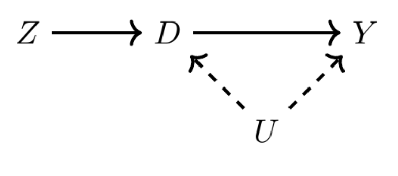
\(Z\) is the instrumental variable

\(D\) is our main variable of interest

\(Y\) Is our outcome variable

\(U\) is unobserved variables.

So what is this saying? \(Z\) varies, \(D\) varies, which causes \(Y\) to change. Ok, so what? Why do we need \(Z\)? Can’t we just look at the effect of \(D\) on \(Y\), controlling for other variables? We could, but remember that \(U\) is unobserved variables,

Requirements for Instrumental Variables

There are two essential requirements for an instrumental variable. You must satisfy both conditions; however, as we will see, the second condition is quite difficult to justify. The two critical components are: 1) the instrument must be related to our X (variable of interest) and 2) must satisfy the exclusion restriction.

Condition 1: Instrument relates to X

\[ Cov(z,s) \neq 0 \]

\(Z\) needs to influence \(s\) (remember \(s\) is the notation we are using for main variable of interest). All this is saying, is that \(Z\) needs to influence \(s\)!

If \(Z\) does not change \(X\) then that means it does not change how the treatment is assigned. This is a non-starter and if we can’t do this, then we don’t have a good instrumental variable. This assumption is testable and is fairly straightforward. It is the easiest part of your IV setup to defend, since it requires a simple regression of your X on Z.

Condition 2: Exclusion restriction

\[ Cov(z, \epsilon) =0 \]

This is where instrumental variables usually get taken down. And for this assumption, you have to defend theoretically - you cannot “prove” you have satisfied the exclusion restriction. The exclusion restriction states that your instrumental variable must not be correlated with your \(y\). This is somewhat of a misnomer, your \(Z\) can be correlated with \(Y\) but only through \(X\) (in the example DAG above, \(X\) is \(D\)).

What is the perfect instrumental variable?

Think for a second about this. Remember why we are using an instrumental variable in the first place.

A perfect instrumental variable is just a variable that perfectly randomizes the assignment of our treatment! A random number generator is technically an instrumental variable. It relates to X by assigning some people to different levels of X. Further, it does not relate to Y (or at least only relates to Y through X). Always remember the goal for causal inference with observational data: we want our treatment variable assignment to be as close as possible to random assignment. We can’t control the assignment, so we have to be creative!

Some popular instruments you may encounter

Some instruments I have come across in the discipline. Whether you think these are good instruments is up to you. I am merely documenting them.

Rain

There is perhaps no more popular instrumental variable than rain. Rain is the quintessential instrumental variable. I have seen it used extensively in papers related to voter turnout.

Distance

This IV may exist in different forms. In any sense, it generally refers to proximity, or the distance from some thing. Below I provide an example of distance as an instrumental variable. This example uses David Card’s famous estimation of the causal effect of education on earnings. Card uses proximity to a university as the instrumental variable. The paper can be found [here].

Waterways

Waterways was an instrumental variable I came across in Jessica Trounstine’s book: Segregation by Design: Local Politics and Inequality in American Cities.

Altitude

Altitude was an instrumental variable I came across on another individual’s research at an APSA panel.

Compliers in an instrumental variable setup

Now that we have a decent understanding of what an instrumental variable is doing, we can complicate it a little more. Remember that we want to argue our instrument variable is exogenously assigning the treatment and they gets us closer to being able to argue our treatment assignment is as-if random. BUT, there may be heterogeneous effects of that instrument variable on different people. That is, the instrument may be valid for determining the treatment status of some individuals but not others. You should think of these as compliers. What are the different ways someone may receive the treatment? Possible groups include:

• Never-taker - never receives the treatment, regardless of the assignment status

• Always-taker - always in the treatment group, regardless of the assignment status

• Complier - Gets the treatment when assigned to the treatment group; does not get the treatment otherwise

• Defier - Always does the opposite of assignment: does not get the treatment when assigned, but does get the treatment when not assigned

For example, imagine we want to know the causal effect of education on earnings. Now, you might recognize the problem with this, education is endogenous to earnings. People choose their level of education for a variety of observed and unobservered reasons. We cannot randomly assign people to different levels of education, so we must try to find an instrument if we want to know the causal effect of education on earnings. One candidate instrument is proximity to a 4-year university. If this setup sounds familiar, it is because it is the instrument Nobel prize winning economist, David Card used for this same question. Like a good student of econometrics, you are probably struggling to understand how this might be a good instrument. There are many reasons to be skeptical of this instrument in regards to satisfying the exclusion restriction.

Card goes on to defend the instrument’s validity, but he makes an important distinction in regards to men from poor families. He argues the instrumental variable identifies the causal effect for the marginal student. Men from less-educated or poor families are more sensitive to college proximity. These individuals are the marginal compliers who drive the IV estimate. His point here is that men from poorer backgrounds are less likely to endogenously sort into these areas, that conditional on other variables, the proximity to college exogenously assigns their level of education. For this group, proximity to college randomly assigns the level of education. The use of the instrument is to make the argument that for this group of men, the treatment is effectively a random assignment and allows us to isolate the causal effect of education on earnings. Card has estimated the Local Average Treatment Effect (LATE). The point here is that the instrument only credibly determines the treatment status for some group of people. In Card’s case, the instrument is valid for individuals from poor families but not for wealthier families. Card hedges his language a bit here, but note that you need to further defend this assumption, which requires additional defense and argumentation. For this example, do you actually believe proximity to college is assigned as-if random just for men from poor families?

The pitfalls of instrumental variables

In my opinion, instrumental variables are quite convincing in theory. However, they start falling apart pretty quickly in reality. Some researchers think finding a useful instrumental variable is impossible. I am somewhat agnostic to that point. I think the main issue with instrumental variables is not necessarily because that they tend to violate the exclusionary principle in some way, but rather because they muddy our story. It is really hard to find a good instrumental variable. Reviewers and readers alike will usually latch on to your instrument and attack it relentlessly. When IVs get used in research, the researcher has to spend considerable time arguing about why their instrument is a good instrument. If you read the paper I discuss below using puberty as an instrument, you will see what I mean. In my opinion, this long diatribe starts to muddy the focus of what we are actually interested in and is the major reason why instrumental variables are frowned upon. They turn into a paper that just ends up being a defense against critiques of why the instrumental variable they chose is not problematic. In any sense, the vibe I get is that political science is not super into instrumental variables, while economist are a bit more into them, but even they have some considerable debates about their validity.

Writing a research paper with an instrumental variable

Example paper: Early Marriage, Age of Menarche, and Female Schooling Attainment in Bangladesh. Erica Field & Attila Ambrus

Abstract:

Using data from rural Bangladesh, we explore the hypothesis that women attain less schooling as a result of social and financial pressure to marry young. We isolate the causal effect of marriage timing using age of menarche as an instrumental variable. Our results indicate thateach additional year that marriage is delayed is associated with 0.22 additional year of schooling and 5.6 percent higher literacy. Delayed marriage is also associated with an increase in use of preventive health services. In the context of competitive marriage markets, we use the above results to obtain estimates of the change in equilibrium female education that would arise from introducing age of consent laws.

Question:

Do women in rural Bangladesh attain less schooling because of pressures to marry young?

Instrumental variable:

Menarche - the age of the first menstrual cycle

Why the need for an instrumental variable?

Statistical evidence indicates that women who marry young fare worse. However, it is difficult to assess the extent to which these outcomes are driven by the timing of marriage as opposed to common factors related to poverty and traditional gender views that also hinder female advancement.

Child marriage is most common in impoverished and culturally traditional settings. The observation that women who married young have on average less education does not imply that forcing girls to postpone wedlock would improve their outcome.

Breaking this down:

The authors want to know if early marriage causes less education. The problem: early marriage and less education are confounded by low income and traditional values. There are unobservable differences in family background influencing both adolescent maturation and adult outcomes.

Let \(X\) is the age of the girl when she is married.

Let \(Y\) be educational attainment of the girl.

Authors want to show that the lower \(X\) is, the less education the girl will receive. Perhaps we can control for income, but we cannot really control for traditional values. As such, the age of marriage is not a random assignment, it is influenced by rates of income and traditional values. So we need an instrument that helps us assign the X as-if random. There is a strong incentive to marry daughters as young as possible; however, girls in Bangladesh are typically withheld from the marriage market until the onset of puberty.

They argue: “In particular, natural variation in the timing of first menstruation within athe age range of 11-16 generates quasi-random differences in the earliest age at which girls are at risk of marrying.”

What the authors need to show:

1. They need to show that age of first menstrual cycle relates to the age of marriage.
2. The age of menstrual cycle has no effect or does not relate to education attainment.

Motivation:

• Girls drop out of school much higher than boys.

• early marriage is a big reason

Estimation Strategy

• Age of first marriage is traditionally bounded below menarche, these differences generate exogenous variation in girls’ risk of marrying young.

\[ Y_i=\alpha_0+\alpha_1A_i+\alpha_2'X_i + \upsilon_i \]

Where \(Y_i\) is the outcome of interest, \(A_i\) is individual \(i\)’s age at marriage, and \(Z_i\) is \(i\)’s age at menarche. \(X\) includes the following set of controls: adult height, family background and family composition characteristics, religion, and a dummy variable indicating whether the women currently resides in a district of Matlab that is part of the treatment region for the national fertility intervention.

So above we have the regression but as we know, age of marriage \(A\) is influenced by unobservable characteristics. So we need a variable that exogeneously influences \(A\). This will be our instrument aka age of first menstrual cycle. Thus:

\[ A_i = \beta_0 + \beta_1Z_i+\beta_2'X_i +\upsilon_i \]

This equation is saying \(A_i\) is influenced by our set of controls AND our instrumental variable: age of first menstrual cycle. Basically:

• Marriage age \(A_i\) varies with the instrument \(Z_i\) (age at menarche).

• AFTER conditioning on controls \(X_i\)

• \(\beta_1\) must be non-zero for the instrument to be relevant.

So does age of menstrual cycle covary with age of marriage? They find it does. This is the first stage regression aka the instrument relates to the variable of interest. Every additional year that puberty is delayed, marriage is postponed an estimated .74 year. These findings are robust under different specifications.

Exclusion Restriction

• The exclusion restriction requires that the relationship between puberty and adult outcomes is fully mediated by changes in age at first marriage, such that delayed marriage is the only pathway though physical maturation influences school.

• This set of evidence suggests that much of the variation in timing of first menstruation is uncorrelated with determinants of adult well-being other than marriage age and that differences in family background according to age of menarche are unlikely to confound the analysis.

Section X: Bias and Efficiency

Bias and efficiency are critical components in how we interpret our results. They have both theoretical and data implications. 333

Bias

When we use data to generate inferences, we prefer those inferences to be unbiased, that is, correct on average. @kkv We generally only get one sample, but theoretically, if we were to do multiple samples, we should expect slightly different inferences but, on average, center on truth. The variation around the true value (which we fundamentally cannot know) should not be systematic. Bias occurs when there is a systematic error in the measure that shifts the estimate more in one direction than another over a set of replications. An unbiased procedure will be correct when taken as an average many applications-even if no single application is correct. Achieving unbiased inferences depends on the original collection of data and its later use. Bias refers to the coefficient, our \(\beta\)!

Bias manifests in our research design and data collection!

An estimator \(\mu\) is said to be unbiased if it equals \(\mu\) on average over many hypothetical replications of the same experiment.

Bias Formally

\[ E(Y_i)=\beta X_i \]

\(\beta\) represents the true effect (the Random Causal Effect in the language of KKV), which we do not observe. But we can estimate \(\beta\) with our realized (observed) estimate of the phenomenon, \(b\). We can estimate \(\beta\) using least squares regression:

\[ E(b) = E(\frac{\Sigma X_iY_i}{\Sigma X^2_i}) \] When you complete solve this equation you will get:

\[ b = \beta \]

meaning that \(b\) is an unbiased estimator of \(\beta\).

Statistical Bias

Substantive Bias

Types of Bias

Selection Bias

Selection bias refers to choosing observations in a manner that systematically distorts the population from which they were drawn.

Any selection rule correlated with the dependent variable attenuates estimates of causal effects on average.

Omitted Variable Bias

Omitted variable bias (OVB) refers to the exclusion of some control variable that might influence a seeming causal connection between our explanatory variables and that which we want to explain.33

We do not need control variables, even if they have a strong influence on the dependent variable, as long as they do not vary with the included explanatory variable.

For you to have OVB, your confounding variable must influence \(Y\) and correlate with \(X_1\)

Signing OVB Table

	\(Corr(x_1,x_2)>0\)	\(Corr(x_1,x_2)<0\)
\(\beta_2>0\)	positive bias	negative bias
\(\beta_2<0\)	negative bias	positive bias

We need to always account for OVB, of course, there may be times we cannot. Perhaps we don’t have that data. While not ideal, this may not be fatal. The table above allows us to think how and in what direction is the exclusion of this control variable biasing our result. We can then infer it’s effect and be clear about it in our results.

Control for everything?

Concern for OVB should not lead us to automatically include every variable with these conditions. In general, we should not control for an explanatory variable that is in part a consequence of our key causal variable.

Other Causes of Bias

Truncation

Truncation is a problem with our sampling (some observations are not sampled).

Truncation can attenuate bias

Censoring

Censoring can also attenuate bias. Remember that censoring is a problem with our measurement (some observations are measured inaccurately

Efficiency

An efficient use of data involves maximizing the information used for descriptive or causal inference. We want to be confident that the one estimate we get is close to the right one. Efficiency provides a way of distinguishing among unbiased estimator.

How do we measure efficiency?

Efficiency is a relative concept that is measured by calculating the variance of the estimator across hypothetical replications. For unbiased estimators, the smaller the variance, the more efficient (the better) the estimator. Our standard errors are directly related to the concept of efficiency. They tell us the certainty of our estimate.

We gain greater efficiency with more observations!

We lose efficiency if we include a control variable that does not influence the DV but is correlated with our main explanatory value, thus leading to a less efficient estimate of the causal effect - chose your control variables carefully!

Example

We can borrow KKV’s example, suppose we are interested in estimating the average level of conflict between Palestinians and Israelis in the West bank and are evaluating two methods: a single observation of one community, chosen to be typical, and similar observations of, for example, twenty-five communities. Efficiency provides us the ability to compare the estimators of these two and which is better. IF applied properly, both estimators should be unbiased, that is, they should center on truth and are not systematically predicted. When we calculate the variance of these estimators, the estimator with one observation will just provide the variance. However, the estimator with 25 observations will be that variance divided by 25, yielding a smaller number. This smaller number translates to a smaller variance and thus a more efficient estimate. There is less variability in our estimator. If we were to conduct the test again, we would likely get a different estimate (due to random error) but, because our variance is low, our estimate is likely to be very close to that original estimator.

Efficiency Formally:

Bias and Efficiency Trade-off

AKA: Bias v. Variance Trade-off; Precision v. TK

To belabor bias and efficiency one more time, it useful to think of any inference as an estimate of a particular point with an interval around it.

When we think of bias and efficiency, we of course want low bias and high efficiency. However, this is not always possible.

I think understanding this trade-off is actually a little bit abstract and does not become clearer until you learn about other models, specifically non-parametric (machine learning) models. In these non-parametric models, we are trying to estimate the coefficient as closely as possible. These models are called “black boxes”. This is because we throw many variables into them (we usually have millions of observations) and they use all that information to make the closest possible estimate. This does have perks, but there is an important sacrifice that occurs in these models. Since these models are maximizing predictions, they tend to overfit. Overfitting occurs when a model starts to memorize the aspects of the training set and in turn loses the ability to generalize. In abstract terms, imagine our simple regression line, in non-parametric models we can allow the line to flex and break and curve based off the of the data, this will yield extremely precise predictions (low bias).

Alternatively, a high bias, but low variance model may be a simple curve/line in a cloud of points. This may seem like regression (to some extent it is) however, the point is that regression is so sought after because it generally strikes that appropriate balance between bias and efficiency.

The goal is more information relevant to our hypothesis: we need to make judgments as to whether this information can best be obtained by more observations within existing cases or collecting more data.

The formal way to evaluate the bias-efficiency trade-off is through the calculation of the mean square error (MSE).

Measurement Error

At first glance, this section may seem out of place. However, measurement (and subsequently measurement error) have important implications for bias and efficiency.

Measurement

When we have settled on a question and selected our observations, our focus then turns to how we measure the concepts we are interested in. How we measure some phenomenon has major implications for the internal validity of our study. If our theory is about democracy, and we include a state like Russia, there is clearly a gap between our theory of democracy and what we measured.

When collecting data we need to focus on two aspects of how we measure:

1. validity
2. reliability

We should always strive to maximize the validity of our measurements. Validity refers to measuring what we think we are measuring. We want our concept to be clean and easily definable so that when we measure it, the measurement is internally consistent with our theory. We do not want other concepts to cloud how we measure it.

We should always strive to ensure that data-collection methods are reliable. Reliability means that applying the same procedure in the same way will always produce the same measure. A reliable measure should produce the same results when applied by different researchers.

Systematic Measurement Error

Systematic measurement error, such as a measure being a consistent overestimate for certain type of units, can sometimes cause bias and inconsistency in estimating causal effects. Any systematic measurement error will bias descriptive inferences. Systematic measurement error which affects all units by the same constant amount causes no bias in causal inference. If everyone in the survey over reports their income earned, the causal estimate of our variable of interest will be the exact same since the error is present across all observations.

But what if there is systematic measurement error in one part of the sample? This is where we start running into problems. When this occurs, both descriptive and causal inference about the causal effect is biased.

Nonsystematic Measurement Error

Random measurement error does not bias the variable’s measurement. Random measurement error means that values are sometimes too high and sometimes too low but correct on average, which can lead to obvious inefficiencies but not bias in descriptive inference. For causal inference, random measurement error can lead to different effects depending on where it is.

Nonsystematic Measurement Error in the Dependent Variable

Random measurement error in the dependent variable reduces the efficiency of the causal estimate but does not bias it. This will lead to causal estimates that are sometimes too large and sometimes too small. The result is that random measurement error in the dependent variable produces estimates of causal effects that are less efficient and more uncertain.

To overcome this, we can improve efficiency by 1) increasing the accuracy of our observations, or 2) increasing the number of imperfectly measured observations in different communities. Both of these options increase the amount of information we bring to this problem.

influences vertical deviations of line!

Formalized Example:

Nonsystematic Measurement Error in the Explanatory Variable

Random error in an explanatory variable can also reduce the efficiency of the causal estimate but can also produce bias in the estimate of the relationship between the explanatory and dependent variable. The bias this measurement error produces results in the estimation of a weaker causal relationship than is the case. It is biased in the direction of zero or no relationship.

Practical Guidelines for Measurement Error in the Explanatory Variable:

1. If an analysis suggests no effect to begin with, then the true effect is difficult to ascertain since the direction of bias is unknown; the analysis will then be largely indeterminate and should be described as such. The true effect may be zero, negative, or positive, and nothing in the data will provide an indication of which it is.
2. However, if analysis suggests that the explanatory variable with random measurement error has a small positive effect, then we should use the results in this section as justification for concluding the true effect is probably even larger than we found. Similarly, if we find a small negative effect, the results in this section can be used as evidence that the true effect is probably an even larger negative relationship.

Section X: Natural Experiments

Natural experiments are experiments where the researcher does not exercise control over how the treatment is assigned. In short, nature assigns the randomization. These class of research has a lot of ‘cache’ and is quite fun to read. In my opinion, people like these types of experiments because they usually leverage some ‘odd’ thing that happened in the world to estimate a causal effect. However, these experiments suffer a bit because you will have to explain and defend how nature randomized the treatment. There are different flavors of natural experiments, some are good and some are not so good. I will discuss those here.

Section X: Diff-in-diff

Literally standing for the ‘differences in the difference’, diff-in-diff is a common natural experiment framework model you will come across. The framework is somewhat straight forward; some exogenous event occurs, which is assigned to a certain population, leading to some outcome \(y\). Since we want to estimate a causal parameter, we need a counterfactual. In diff-in-diff, we are going to make an argument that we our counterfactual is similar to those that got treated, and the effect of our variable of interest is the difference in effect in our population over that time period compared to the difference in population that did not get the treatment. The difference of these two is our causal effect of \(x\), thus the ‘diff-in-diff’. As with all of our models, we do need to make assumptions.

Assumptions in diff-in-diff

For this to work, you must be able to identify a suitable comparison group.

Your comparison group is the same in everything else and the only difference is that they did not receive the treatment. They represent your counterfactual. Your treatment group would have had the exact same trend that your comparison group had, if they did not receive the treatment.

The most critical assumption made in a diff-in-diff is the ‘equal trends assumption’. You cannot prove you have satisfied the equal trends assumption. The equal trends assumption is an assumption that you can provide support for, but ultimately, you cannot completely satisfy it. You are trying to convince the reader that assumption you have made is reasonable.

Equal trends and Constant Treatment Effect (ATE)

The equal trends assumption (also colloquially called the parallel trends assumption) is what will give you the causal estimate of your treatment. You cannot prove you have satisfied this assumption. In simple terms, the assumption is that had no treatment occurred, the gap between treated and untreated groups would have remained constant. The critical component of this design is to use the change in the untreated group to represent all non-treatment changes in the treated group. You need to argue that the only reason for the diverging trends was a result of the treatment group receiving the treatment.

So what do we do to help us argue in favor of the equal trends assumption? We can test prior trends, that is, did the treatment group and the untreated groups, have similar trends in the period before the treatment? If they were, this gives credibility to our parallel trends assumption (IT DOES NOT PROVE THE ASSUMPTION).

Writing a diff-in-diff paper

Defend against the “Ashenfelter dip”

Extensions of diff-in-diff framework

The following frameworks are extensions to the simple diff-in-diff. These will be fairly similar with a slight variation. Our choice to use these will depend on our theory and the nature of our data. I don’t go in depth here, these are just to expose and introduce extensions and their subsequent logic motivating their existence.

Triple Diff-in-diff

In our estimate of the diff-in-diff, we use an interaction to estimate the causal effect. In the triple diff, we do the same thing, but add another interaction to that previous interaction. In a nutshell, it is a three way interaction.

For example, perhaps we have already estimate the effect of the diff in diff. But now we are interested in knowing if this effect is conditional on income level. A triple diff is simply this. We are going to test if this effect is conditional. Thus, we are comparing how low v. high income differs in the treated group relative to how they differ in the control group. But the mayor also hires a new DA, potentially confounding our treatment effect.

Placebo Analysis

In a placebo analysis, we are doing the exact same thing as a diff-in-diff, only we change our outcome variable to something else. Only, we hope for null results. The logic here is straight forward, we are testing the effect of X on a different outcome variable that should have no effect. Say we are interested in the effect of the mayor hiring more police on crime rates. But the mayor also hires a new DA, potentially confounding our treatment effect. Hiring more police unlikely to affect tax fraud, but if new mayor hires more police and replaces DA, both outcomes could be affected. So we run our placebo analysis of hiring more police on our new (placebo) outcome variable: tax fraud. These two should be unrelated, if they are related, this implies we have a violation of our parallel trends assumption due to other contemporaneous changes.

Is my treated effect picking up the true effect or is it just picking up correlated noise? Remember that our goal is to show that these two groups would have the same trend had one of them not received the treatment. When we use a placebo, we are testing an outcome that should not respond to our treatment. If it does, this means our model has some omitted variable and that your treatment variable is not the causal effect but actually correlates with some other unobserved variable. In simpler terms: if the diff-in-diff shows a treatment effect on the placebo, then:

1. that treatment effect must be coming from something other than the treatment
2. therefore, the treated and control groups must have different trends, violating our parallel trends assumption.

Synthetic Diff-in-diff

This one is quite statistically ‘progressive’ - it’s a bit magical. A synthetic diff-in-diff is used when we do not have an obvious counterfactual (an obvious comparison group) to conduct our normal diff-in-diff. So what do we do? Well, we synthetically create a control (comparison) group. This method uses a lot of statistical modeling to estimate how best to construct this group. This synthetic group will be constructed from “donor data”. We will use donor data that is similar to the treatment group in every way, but since they did not receive the treatment, they will differ only in that variable. This will hinge entirely on how we tell the model what variables to estimate on to construct the synthetic comparison group. Let’s work through a quick example.

Perhaps we are interested in understanding the effect of of governmental ‘handouts’ on the employment rate. One theory is that more governmental assistance will decrease employment, since they now have more money supplanted by the government. Or it is possible, that more money may have no impact on employment rate and actually increase economic output since that money increases the spending power, potentially increasing jobs needed; more money -> more demand -> more jobs needed. How can we figure this out?

Luckily, Alaska provides a unique research opportunity to study this exact question. In 1982, all Alaskans began receiving dividend checks from oil revenue occurring in the state. This treatment is a great one theoretically to help us answer the question we outlined above; however, we have a technical problem, if we want to estimate the causal effect, who do we compare Alaskans to? While they are American, a comparison of any state to Alaska will be tough given how much different Alaska is. And since, all Alaskans received the dividend, there is no sub-population within Alaska to use as a comparison group. What do we do? We construct a synthetic Alaska.

We are going to construct synthetic Alaska from donor data. This donor data will be individuals from other states. We are basically going to match that donor data with Alaskan data on specified covariates. We are making a fake Alaska that resembles the true Alaska as close as possible. Importantly, we choose the covariates to ‘match’ to, how do we this is researcher defined and thus must be justified and defended. We still make the same equal trends assumption, and our synthetic data should have parallel trends extremely similar to the true Alaska. Since, our synthetic data does not include the treatment variable, we are able to compare the treatment effect in the diff-in-diff between real and synthetic Alaska.

In simple terms, the structure of a synthetic diff-in-diff is as follows:

1. Setup: Natural Experiment with a single treated group.
2. take obs from donor pool -> created weighted average of donor pool then use as counterfactual.
3. Algorithm will pick what observations to pick from donor pool (you decide what variables)
4. Make sure it worked (check equal trends assumption) - note a synthetic diff in diff will have very similar equal trends.
5. Now just do a regular diff-in-diff.