
# compare what happens when we increase n.
p <- seq(0,1,by=0.01)
l <- (p^2)*(1-p)^3
plot(l ~ p, type="l")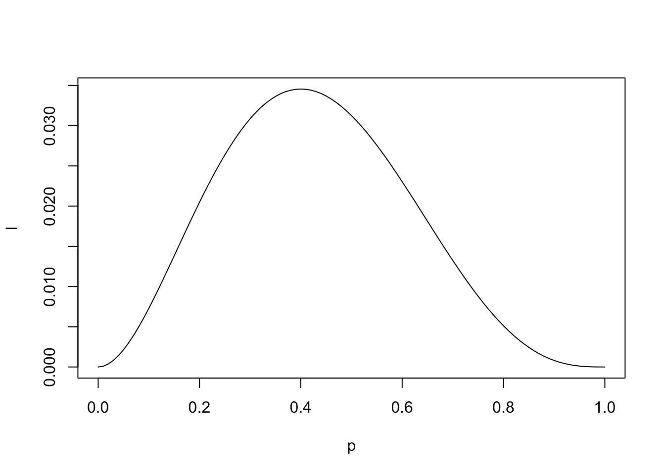
p[which(l == max(l))][1] 0.4p <- seq(0,1,by=0.01)
l <- (p^40)*(1-p)^20
plot(l ~ p, type="l")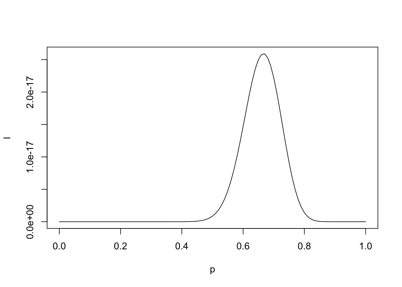
p[which(l == max(l))][1] 0.67Introduction of the book. Political science methodology is disjointed and not as completely coherent as it should (and needs) to be. King seeks to organize and centralize the political science methodology.
Statistic Model: a formal representation of the process by which a social system produces output.
Inference: the general process by which one uses observed data to learn about the social system and its outputs.
Estimation: the specific procedure by which one obtains estimates of features (usually parameters) of the statistical model.
The important question for political science research:
is the underlying process that gives rise to the observed data
What are the characteristics of the social system that produced these data?
What changes in known features of the social system might have produced data with different characteristics?
What is the specific stochastic process driving one’s results?
By posing these questions, statistical modelling will be more theoretically relevant and empirically fruitful.
Conditional probabilities: describing the uncertainty of an observed or hypothetical event given a set of assumptions about the world.
Likelihood: a measure of relative uncertainty
Summary: Run models that find parameters that are most likely to have generated the observed data.
These models are hard to interpret.
Goal: Familiarize you with a variety of MLE models used in the social sciences.
Probability has to sum to 1.
Probabilities are:
Bounded between 1 and 0.
Sum of probabilities equal 1.
Trials -> \(\infty\)
Mutually exclusive outcomes (Independent).
Theta is the only parameter we need to estimate.
We are still specifying the distribution of the outcome variable. Is it a poisson, bernoulli, normal, etc?
L stands for “likelihood function”
Our goal is to select some \(\theta\)* -> \(\hat{\theta}\) as to maximize the likelihood of these data being generated. Ways to do this:
plug in candidate \(\theta\)* values
look at the graph
optimize function (solve for \(\theta\)*)
No priors! (that would be Bayesian)
for our coin flip example, we know .5 is the probability but we only have a set of {H,H,T}
Without anymore knowledge, the best estimate of \(\theta\) is 2/3 or .66.
We use ML anytime our dependent variable has a distribution that was not generated by a Gaussian (normal) process.
see slide 23 for examples.
We can estimate all of these using OLS but we may hit a few snags and violation assumptions.
Working through an ML problem is as follows:
Build a parametric statistical model
Define the probability density for \(Y_i\) (uncertainty component)
Define the systematic component (\(\theta\))
Maximize the likelihood function, given the data.
Interpret
We will pretty much always use log-likelihood.
why?
logarithms turn multiplication problems into addition problems.
likelihood starts to breakdown around N=1000. Log-likelihood does not. Why?
Our optimization function is multiplying probabilities
what happens when we multiply a bunch of probabilities?
# compare what happens when we increase n.
p <- seq(0,1,by=0.01)
l <- (p^2)*(1-p)^3
plot(l ~ p, type="l")
p[which(l == max(l))][1] 0.4p <- seq(0,1,by=0.01)
l <- (p^40)*(1-p)^20
plot(l ~ p, type="l")
p[which(l == max(l))][1] 0.67Probability = we know which universe we are in, and the probabilities of all events in that one universe add up to 1.
area under a fixed distribution
Likelihood = we know what we observed, and we consider the probability of what we observed in any possible universe.
\((\theta|y_i)=Pr(y|\theta)\)
you have to pick which distribution generated y.
Remember:
Traditional probability is a measure of absolute uncertainty. It comes from three axioms:
However, the likelihood is only a relative measure of uncertainty.
Likelihood model is never absolutely true. It is assumed. We always have to assume a probability model.
Therefore, we assume that information about \(\theta\) comes from
the data
assumption about the DGP (assumed probability distribution)
Important to assume outcomes are independent.
Pick a theta and figure out the probability/distribution of outcomes.
Whath happens when we multiply a bunch of probabilities together?
they get really small
so we use logs.
what happens when we take natural logs of probabilities?
we get negative numbers - and they will become more negative with more observations.
take value closes to zero
We are calculating the derivative of the highest point of the joint distribution.
Types of optimization methods:
Numerical
grid search: Give me a bunch of plausible values of theta and evaluate.
we will find a global maximum.
very slow
computationally becomes crazy very quickly.
Iterative
this is the “default” one - everyone does this.
Others…
We have discussed how to obtain the MLE, \(\hat{\theta}\). Yet it is an estimate.
uncertainty is kinda measured by the curvature.
standard errors are derived from the negative of the inverse of the second derivative.
standard errors can’t be negative
bigger values imply smaller variance.
bigger negative = more curvature. see equation 8/9 on slides.
we take take the inverse since larger (more negative) values indicate a sharper curvature, which indicates more certainty in our estimate.
We use the Hessian for standard errors in MLE.
Variance = \(-[\textbf{H}^-1]\)
SE: \(\sqrt{-[\textbf{H}^-1]}\)
Sufficiency: there exists a single \(\theta\)
Consistency
Asymptotic normality
Invariance: ML estimate is invariant to functional transformations.
Efficiency: MLE has the smallest variance (asymptotically), as given by the Cramer-Rao Lower Bound
small sample issues. Since ML is asymptotically normal, use Z- rather than t-statistics.
We know the VCV is biased in small samples
(not a disadvantage) but most MLE models use z rather than t-stat.
Have to make distributional assumptions. We must characterize the nature of the statistical experiment.
some regularity conditions must be met.
Provides goodness-of-fit with penalization for model complexity
Used for feature (i.e., covariate) selection
Relative, not absolute.
Data-dependent (sample-dependent, just like log likelihood): numerical values of Y must be identical.
No hypothesis test
Akaike Information criterion (AIC)
\(AIC=2k-2ln(L)\)
Lower AIC is preferred model.
Schwartz Bayesian information criterion (SBIC)
\(SBIC=ln(n)k-2ln(L)\)
Lower SBIC is preferred model
stronger penalty for over fitting than AIC. Penalty derived from “prior” information.
AIC AND BIC ARE NOT TESTS THEY ARE VALUES
Restricted Mode: Less parameters
unrestricted model: all parameters.
likelihood ratio test basically tells you if there is statistically significant difference between two models
complex v. simple
Lots of tests for additional “nuisance” parameters
Reject H_0: restricted parameter sufficiently improves model fit; should be unrestricted
Fail to reject H_0:
Similar to LR tst,
only estimate unrestricted model.
if MLE and the restriction are quite different, W becomes large.
reject: parameters sufficiently different from the restriction
LR-Test requires estimating two models; may be computationally intensive
LM -Test requires estimating only a restricted model. Yet finding MLE of constrained model is sometimes difficult. Some LM derivations get around this.
Wald requires estimating only an unrestricted model. Can also test non-linear restrictions.
All are asymptotically equivalent
In small samples, LM is most conservative, then LR, then Wald.
When doing these in code just keep track of which is restricted and unrestricted.
GLMs are generalized version of linear regression.
basically just a bunch of different link functions
GLMs are linear in parameters.
Basic order:
figure out what DV is
pick a distribution (based on DV)
Begin by specifying the random (stochastic) component.
Normal:
mean, media, and mode all occur at \(\mu\)
The distribution is symmetric about \(\mu\) (eliminate any random variable that is skewed)
Distribution is continuous on the real-number line (eliminates any discrete random variable or bounded random variable)
central limit theorem
mean and variance are separable
Most distributions are not normal!
MLE uses z-statistics because it is asymptotically normal.
\(\sigma^2\) is not usually reported. It is an ancillary parameter.
do likelihood test
rho is the correlation coefficient of epsilon and its prior value.
when you take the lag of a series the first observation goes away.
censoring changes shape of the distribution, truncation does not change the distribution for the un-affected range.
Both cause bias (attenuation) and inconsistency. More data does not help us here!
Censoring
Censoring is a symptom of our measuring
is in sample (just a discrete value though)
“values in a certain range are all transformed to (or reported as) a single value”
income in surveys often censored ($250,000 or more) since there are so few individuals that would comprise these categories
ex: if an individual on a survey responds 1, they are a strong democrat, 2,3,4, weak affiliation/independent, 5, strong Republican.
This results in lumping/bunching near the censoring point \(\tau\)
Estimates are biased (attenuated) since observations farthest from the center of the distribution are restricted to some arbitrary upper (lower limit)
Three types:
left (lower) censor
Right upper censor
Interval censor.
We have an observation in the region somewhere…but we don’t know exactly what the true value is”
Dealing with Censoring
Truncation
truncation effects arise when one attempts to make inferences about a larger population from a sample that is drawn from a distinct sub-population.
Theory will tell you where the truncation is. To fix truncation, you have to know you have truncation.
Truncation is a symptom of our sampling
Observation? what observation?
produces bias
moves mean away from tau
shrinks variance too
sample selection is a form of truncation
This is in my Y.
Examples: data on GDP of countries from the World Bank (excludes those that are too poor to report data from their statistical agency)
Dealing with Truncation:
truncated normal distirbutions are not full probability distributions since the area under the curve (the CDF) does nto sum to one
thus we cannot form the likelihood function.
Sample Selection Bias
a type of truncation
nonrandom sampling of observations.
incidental truncation (truncation caused by some other variable, not y itself)
What’s the population we are generalizing to?
Selecting on the DV
sample selection bias is not the same as selecting on the DV.
Sampling on DV means deliberately choosing certain y outcomes.
Discrete outcomes
We can estimate \(\pi_i\) using OLS.
\(\pi_i = X_i\beta\) using OLS
benefits:
linear interpretation of betas
simple…much faster since using OLS
Works well if \(X_i\) is also distributed Bernoulli
Drawbacks:
“impossible” predictions; probabilities exceed 0 and 1.
censoring issue.
error not normally distributed.
error will not have constant variance.
LPM is not ideal but its not terrible. You can run it sometimes. What we want is
\(\pi_i=g(X_i\beta)\)
we can first express \(\pi_i\) as odds
approach infinity in the positive direction
approach zero
logit(\(\pi_i\)) < 0
creates a sigmoid curve.
near inflection point of zero
we are solving for \(\pi_i\)
GO THROUGH SLIDE 17!
constant shifts the inflection point in logit.
big coefficients should have steeper slopes.
if X is smaller, we get a more stretched out curve.
z-score usage
different link function
coefficients in probit model show the increase/decrease in the z-score in response to a change in \(x_ik\)
probit usually steeper but not always
Logit more common in poli sci.
Do not compare logit or probit coefficients - they are different.
think of our Xbetas as a unbounded latent variable
slide 28.
There are several psuedo R^2 measures used for fit of logit/prboit models.
kinda useless. They aren’t exactly R^2.
no need to report really.
AIC/BIC more important.
Signs matter
magnitude less so…
Interpreting single \(\beta\) can be done, but be careful about predictions, as log-odds are not a change in Pr(y=1)
Example: predict Pr(Farm Laborer)
Odds = 1 mean increase in x does not make Pr(y_i =1) more or less likely
odds < 1 mean increase in X makes Pr(y_i) less likely
cant say probability but how much more likely you are to be a farm laborer.
ODD RATIO SHOWN (this is what we should say when we report this).
predictions always depend on the value of other covariates. see slide 37.
How much does Y change given a change at X.
First differences in the logit/probit context do not have all the properties listed previously
first-differences for logit are given by: see slide 40.
critique of expected values/expected change: “we are not aware of any theories that are specifically concerned with 48-year old white women who are independent politically and have an in income of $40k - $45k.
Instead of setting X, we keep all X_i’s at their observed value for each observation, and fix our variable of interest to some value, giving us an expected value for each observation.
Growing use of simulation techniques designed to show statistical and substantive significance of the results.
Typically used to make predictions of Y.
hetero can lead to inefficient estimates in OLS,though coefficients remain unbaised
often worse in logit and probit models, leading to inconsistent estimates
we can model out hetero through ‘robust’ standard errors
or better? if we suspect determinants of hetero, we can model error variance directly through a hetero probit.
use probit for hetero stuff
We are estimating \(\tau\) cut points.
Why do we this over OLS?
It is just a generalization of the logit/probit to accommodate multiple cut-points.
trying to find betas and taus such that we are maximizing our probability that this observation is a 1 (or 2, 3,etc - dependent on category).
Why would I ever run MLE over OLS - this is a comp question
if cut points are equidistant - just run OLS
these are good with vote choice models.
We get log odds when running this
and cut points
Conceptually, when we plug in values and multiply by the coefficients estimated - we get a value that will tell us where the output falls in relation to the estimated cut points (\(\tau\)).
How are Taus getting estimated?
Code needs to use clarify - Andy hasn’t done that yet.
i.i.a is important. - need to know it better.
we are like basically modeling a rate (count/exposure time)
What if we observed multiple bernoulli trials over time?
by definition, these data are truncated at 0.
log count.
think about time. We are segmenting time and seeing the Bernoulli trial with that increasingly smaller time segment.
Poisson function does this.
lambda in our example is the expectation of the # of job changes over 5 years.
y=2 because i wanted to the know the probability you had 2 job changes.
Example: Prussian soldiers who died after being kicked by a horse.
count data is a time story and is almost always not independent.
only used count data when you are pushed up to zero.
when your count data is far from zero, then you prob don’t have to use count models.
IRR
substantively show you the change in counts.
concerned about overdispersed
mean < variance
basically outliers
If variable is overdispersed, it was not generated via a Poisson process.
i mean you can always run a negative binomial and its best if you have overdispersion but if you don’t then poisson is basically better.
change in log-count
Still use clarify.
first difference
irr means count doesn’t move up and down.
if alpha is zero - run poisson.
null is poisson.
Recall: we use anytime we suspect that the data are from a Bernoulli random variable with a large number of trials, with a very low probability of an “event” occurring.
What if our model has a substantial amount of zeros?
mean will shift to the left of the zero.
we need to figure out if we have lots of zeros which is hard
depends on theory
see Netflix example.
poisson is negative binomial when alpha is zero.
One way of modeling zeros is to envision two regimes.
What is \(F\) ? -one of the Bernoulli link functions.
Joint probability
variance is higher than conditional mean
overdispersion
do you have overdispersion or excess zeros?
lots of debate.
Poisson vs NB?
ZIP vs. ZINB
Vuong test - bunch of issues with it.
See protest question on midterm
we don’t observe zero.
these assume that there is a unique DGP that determines whether we observe a zero or truncated Poisson
confusing
The key focus is on the time until an event occurs
Originates from epidemiology where observations were patients, the start was the onset of the study, and th event was death, disease, recovery, etc.
Differs from event count models; we’re now trying to see how long until a single event occurs.
1=failure, 0=no failure
presence of time-varying covariates is going to influence how we structure our dataset.
Epidemiology loves this, poli sci not so much
the proportion/percent surviving is on the vertical axis
time is on the horizontal axis
Data consist of a cross-section of i units
units enter at \(t_0\)
How does \(x\) affect \(T_i\) ?
not a normal distribution!
Weibull, exponetnial, Gompertz
Add in explanatory covariates
Can either be constant across t, or time-varying, depending how the data are structured.
Semi-proportional model:
you don’t have to specify the hazard.
Cox proportional hazard model
whats the probability that a unit fails in the next period
As the time interval between periods, \(\delta\), gets smaller and smaller, we approximate the hazard rate
the hazard rate is the rate at which units fail after time t, given that they have last up to time t.
Exponential is “memoryless”
this means that there is a constant risk of failure at all times.
The most general one
look at gamma first and test down basically.
For most models, such as the exponential and Weibull, the metric output is in proportional hazards.
a one unit increase in x makes the instantaneous rate of failure twice as likely..
It allows users to avoid explicitly specifying the baseline hazard
We don’t care about the baseline hazard (often, since we only guess at what it might be)
We just want to see how covariates affect the hazard rate
Assumption
covariates affect the relative risk of failure, not the shape of the overall hazard function
f(t) was the probability distribution of failure. At what time does our observation fail.
h(t) was the hazard rate; given that an observation has surived to time t, whats the instantaneous rate of failure?
Need to probably know the hazard rate formula
Hazard function is the ratio of the PDF of the failure function over the survivor function.
Cox Model need to be worried about proportional hazard models!!!!!!!
proportional hazard?
Cox model implicitly assumes that the effects are constant (proportional) across time
Need to assume affect of X is the same across time
if this is met you satisfy the proportional hazard.
Another way of thinking about htis is that the coefficients do not change w.r.t. time (since the hazard is some function of time)
The log likelihood function of the Cox model - think of it between actually failed and at risk of failiure. We want to maximize the difference between the two.
we have assumed our coefficients, x, are constant over time within an individual.
However, some may vary over time.
Dont get this confused with time-varying coefficients!
g(t) is effectively a fix for proportional hazards
These help us assess whether PH is violated.
want these residuals to be flat
look at exponential coefficient.
above 1 quicker, lower than 1 slower. see R code.
Respondent chooses not to answer a question about their race/ethniciy
Venezeula fails to report inflation data for 1980 to IMF
Missingness in the DV is not a big problem.
Missingness that may occur is missing completely at random
this almost never happens
If have MCAR, we still have an unbiased estimate of \(\beta\)
Hardest to achieve
Missing at random
weak
means that a missing y variable is not determined by y.
We don’t observe a respondent’s views on abortion if they have a high school level of education or lower
we have another variable that kind of explains the missingness of another variable.
will produce biased estimates unless using FIML
Another weak form of missingness is known as missing not at random
this is bad!
Also called observed at random (OAR), or non-ignorable non-response
i.e. we don’t observe a respondent’s views on abortion if they have particular strong (pro or anti) views on abortion.
we need to know where our missingness is!
we normally do listwise deletion - also called complete-case analysis.
you could fill it in but its really just noise. It’ll effectively be our \(\hat{y}\)
its just not really a big issue
Another way of handling data is interpolation
assuming time series data, we might perform linear model interpolation
whats a good guess of Y, the time before it and the time after.
hard to do outside of time series
will reduce variation
When data are at the end/beginning of a series, they are sometimes extrapolated
filling in values at the beginning or end of a series.
seems a little dodgy
Imputation allows us to fill in missing data, but preserve the inherent uncertainty associated with the filled in value.
Amelia package by King.
Listwise deletion standard errors are bigger than they probably should be
interpolation smaller they should be
imputation probably where SE should be.
the results are not specific to the model you estimated.
Even if i violate assumptions ill still get same results
your model doesn’t rely on model assumptions
Read Robustness Tests for Quantitative Research
why do people run OLS over others?
Andy’s definition:
Do your findings (magnitude, direction and statistical significance) change under differing assumptions?
assumptions: identificiation assumptions, measurement assumptions, estimator assumptions
identification:
Robustness is NOT ensuring the model is well-specified. It starts with the assumed model you chose and builds from there; you’re not going to show a bad model to begin with.
Robustness is not about predictive ability or forecasting.
Robustness checks are a way to check for internal and external validity, but id be wary about saying the model is valid just b/c its robust.
Are our models ever correct?
What are robust standard errors:
changing standard errors
another name: heteroskedastic consistent standard errors
standard errors are consistent even with heteroskedasticity
even if we violate spherical assumptions, standard errors will still be correct
does not alter our \(\hat{\beta}\) ’s, but makes our standard errors “robust to” certain misspecifications.
sandwich operator
typically standard errors will be a little larger after but more correct.
spherical error violation? Do this.
Cluster-robust:
normally distributed errors is probably going to be violated
standard errors will technically be wrong too
so what do we do?
Model Variation tests
Functional form changes
@online{neilon2024,
  author = {Neilon, Stone},
  title = {MLE - {Data} 3},
  date = {2024-08-26},
  url = {https://stoneneilon.github.io/notes/Comparative_Behavior/},
  langid = {en}
}